Agricultural economy/Description and Emissions/Policy issues: Difference between pages
ElkeStehfest (talk | contribs) No edit summary |
Oostenrijr (talk | contribs) No edit summary |
||
| Line 1: | Line 1: | ||
{{ | {{ComponentPolicyIssueTemplate | ||
|Reference=PBL, 2012; Braspenning Radu et al., 2016; | |||
|Reference= | }} | ||
<div class="page_standard"> | |||
==Baseline developments== | |||
In a baseline scenario, most greenhouse gas emissions tend to increase, driven by an increase in underlying activity levels (This is shown in the figure below for a baseline scenario for the [[Roads from Rio+20 (2012) project|Rio+20]] study ([[PBL, 2012]]). For air pollutants, the pattern also depends strongly on the assumptions on air pollution control. In most baseline scenarios, air pollutant emissions tend to decrease, or at least stabilise, in the coming decades as a result of more stringent environmental standards in high and middle income countries. | |||
{{DisplayPolicyInterventionFigureTemplate|{{#titleparts: {{PAGENAME}}|1}}|Baseline figure}} | |||
==Policy interventions== | |||
Policy scenarios present several ways to influence emission of air pollutants ([[Braspenning Radu et al., 2016]]): | |||
* Introduction of climate policy, which leads to systemic changes in the energy system (less combustion) and thus, indirectly to reduced emissions of air pollutants ([[Van Vuuren et al., 2006]]). | |||
* Policy interventions can be mimicked by introducing an alternative formulation of emission factors to the standard formulations ({{abbrTemplate|EKC}}, {{abbrTemplate|CLE}}). For instance, emission factors can be used to deliberately include maximum feasible reduction measures. | |||
* Policies may influence emission levels for several sources, for instance, by reducing consumption of meat products. By improving the efficiency of fertiliser use, emissions of N<sub>2</sub>O, NO and NH<sub>3</sub> can be decreased ([[Van Vuuren et al., 2011b]]). By increasing the amount of feed crops in the cattle rations, CH<sub>4</sub> emissions can be reduced. Production of crop types has a significant influence on emission levels of N<sub>2</sub>O, NO<sub>x</sub> and NH<sub>3</sub> from spreading manure and fertilisers. | |||
* Assumptions related to soil and nutrient management. The major factors are fertiliser type and mode of manure and fertiliser application. Some fertilisers cause higher emissions of N<sub>2</sub>O and NH<sub>3</sub> than others. Incorporating manure into soil lowers emissions compared to broadcasting. | |||
The impacts of more ambitious control policies ({{abbrTemplate|CLE}} versus {{abbrTemplate|EKC}}) on SO<sub>2</sub> and NO<sub>x</sub>, emissions, and the influence of climate policy are presented in the figure below. Where climate policy is particularly effective in reducing SO<sub>2</sub> emissions, air pollution control policies are effective in reducing NO<sub>x</sub> emissions. | |||
See also the Policy interventions Table below. | |||
{{DisplayPolicyInterventionFigureTemplate|{{#titleparts: {{PAGENAME}}|1}}|Policy intervention figure}} | |||
{{PIEffectOnComponentTemplate }} | |||
</div> | |||
}} | |||
Revision as of 16:34, 15 November 2018
Parts of Emissions/Policy issues
| Component is implemented in: |
Components:and
|
| Projects/Applications |
| Models/Databases |
| Key publications |
| References |
Baseline developments
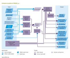
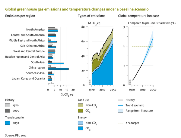
In a baseline scenario, most greenhouse gas emissions tend to increase, driven by an increase in underlying activity levels (This is shown in the figure below for a baseline scenario for the Rio+20 study (PBL, 2012). For air pollutants, the pattern also depends strongly on the assumptions on air pollution control. In most baseline scenarios, air pollutant emissions tend to decrease, or at least stabilise, in the coming decades as a result of more stringent environmental standards in high and middle income countries.
Policy interventions
Policy scenarios present several ways to influence emission of air pollutants (Braspenning Radu et al., 2016):
- Introduction of climate policy, which leads to systemic changes in the energy system (less combustion) and thus, indirectly to reduced emissions of air pollutants (Van Vuuren et al., 2006).
- Policy interventions can be mimicked by introducing an alternative formulation of emission factors to the standard formulations (EKC, CLE). For instance, emission factors can be used to deliberately include maximum feasible reduction measures.
- Policies may influence emission levels for several sources, for instance, by reducing consumption of meat products. By improving the efficiency of fertiliser use, emissions of N2O, NO and NH3 can be decreased (Van Vuuren et al., 2011b). By increasing the amount of feed crops in the cattle rations, CH4 emissions can be reduced. Production of crop types has a significant influence on emission levels of N2O, NOx and NH3 from spreading manure and fertilisers.
- Assumptions related to soil and nutrient management. The major factors are fertiliser type and mode of manure and fertiliser application. Some fertilisers cause higher emissions of N2O and NH3 than others. Incorporating manure into soil lowers emissions compared to broadcasting.
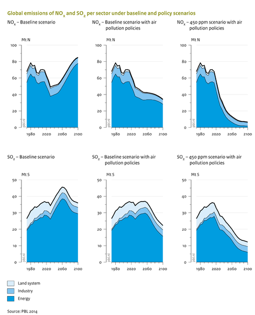
The impacts of more ambitious control policies (CLE versus EKC) on SO2 and NOx, emissions, and the influence of climate policy are presented in the figure below. Where climate policy is particularly effective in reducing SO2 emissions, air pollution control policies are effective in reducing NOx emissions.
See also the Policy interventions Table below.
Effects of policy interventions on this component
| Policy intervention | Description | Effect |
|---|---|---|
| Apply emission and energy intensity standards | Apply emission intensity standards for e.g. cars (gCO2/km), power plants (gCO2/kWh) or appliances (kWh/hour). | |
| Capacity targets | It is possible to prescribe the shares of renewables, CCS technology, nuclear power and other forms of generation capacity. This measure influences the amount of capacity installed of the technology chosen. | |
| Carbon tax | A tax on carbon leads to higher prices for carbon intensive fuels (such as fossil fuels), making low-carbon alternatives more attractive. | |
| Change market shares of fuel types | Exogenously set the market shares of certain fuel types. This can be done for specific analyses or scenarios to explore the broader implications of increasing the use of, for instance, biofuels, electricity or hydrogen and reflects the impact of fuel targets. (Reference:: Van Ruijven et al., 2007) | |
| Change the use of electricity and hydrogen | It is possible to promote the use of electricity and hydrogen at the end-use level. | |
| Excluding certain technologies | Certain energy technology options can be excluded in the model for environmental, societal, and/or security reasons. (Reference:: Kruyt et al., 2009) | |
| Implementation of biofuel targets | Policies to enhance the use of biofuels, especially in the transport sector. In the Agricultural economy component only 'first generation' crops are taken into account. The policy is implemented as a budget-neutral policy from government perspective, e.g. a subsidy is implemented to achieve a certain share of biofuels in fuel production and an end-user tax is applied to counterfinance the implemented subsidy. (Reference:: Banse et al., 2008) | |
| Implementation of sustainability criteria in bio-energy production | Sustainability criteria that could become binding for dedicated bio-energy production, such as the restrictive use of water-scarce or degraded areas. | |
| Improving energy efficiency | Exogenously set improvement in efficiency. Such improvements can be introduced for the submodels that focus on particular technologies, for example, in transport, heavy industry and households submodels. | |
| REDD policies | The objective of REDD policies it to reduce land-use related emissions by protecting existing forests in the world; The implementation of REDD includes also costs of policies. (Reference:: Overmars et al., 2012) | Less emissions due to deforestation and land-use change. |