Energy conversion/Description: Difference between revisions
Jump to navigation
Jump to search
m (Text replace - "ComponentSubDescriptionTemplate" to "ComponentDescriptionTemplate") |
No edit summary |
||
| Line 1: | Line 1: | ||
{{ComponentDescriptionTemplate | {{ComponentDescriptionTemplate | ||
|Status=On hold | |Status=On hold | ||
|Description=The TIMER model includes two energy conversion submodels: the electric power generation model and the hydrogen generation model. Here, the focus is on a description of the electric power generation model ( | |Reference=Hoogwijk, 2004; Van Vuuren, 2007; Hendriks et al., 2004b; | ||
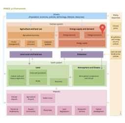
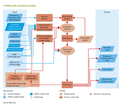
|Description=The [[TIMER model]] includes two energy conversion submodels: the electric power generation model and the hydrogen generation model. Here, the focus is on a description of the electric power generation model (The flowdiagram on the right also shows only the electricity model). The hydrogen model follows a similar structure, and its key characteristics are briefly discussed in this Section. | |||
Electric power generation | Electric power generation | ||
As shown in | As shown in the flowdiagram, two key elements of the electric power generation model are the descriptions of the investment strategy and the operational strategy within the sector. A challenge of simulating electricity production in an aggregated model is that, in reality, electricity production depends on a whole range of complex factors, such as those related to costs, reliance, and the time it takes to switch on technologies. Modelling these factors requires a very high level of detail. Therefore, IAMs such as TIMER concentrate on introducing a set of simplified, meta relationships ([[Hoogwijk, 2004]]; [[Van Vuuren, 2007]]). | ||
| Line 23: | Line 21: | ||
==Fossil-fuel and bio-energy power plants== | ==Fossil-fuel and bio-energy power plants== | ||
A total of 20 different types of power plants, generating electricity using fossil fuels and bio-energy, are included. These power plants represent different combinations of (i) conventional technology; (ii) gasification and combined cycle (CC) technology; (iii) combined heat and power (CHP) and, (iv) carbon capture and storage (CCS) (Hendriks et al., 2004b). The specific capital costs and thermal efficiencies of these types of plants are determined by exogenous assumptions that describe the technological progress of typical components of these plants: | A total of 20 different types of power plants, generating electricity using fossil fuels and bio-energy, are included. These power plants represent different combinations of (i) conventional technology; (ii) gasification and combined cycle (CC) technology; (iii) combined heat and power (CHP) and, (iv) carbon capture and storage (CCS) ([[Hendriks et al., 2004b]]). The specific capital costs and thermal efficiencies of these types of plants are determined by exogenous assumptions that describe the technological progress of typical components of these plants: | ||
*For conventional power plants, the coal-fired plant is defined in terms of overall efficiency and investment costs. The characteristics of all other conventional plants (using oil, natural gas or bio-energy) here are described in the investment differences for desulphurisation, fuel handling and efficiency. | *For conventional power plants, the coal-fired plant is defined in terms of overall efficiency and investment costs. The characteristics of all other conventional plants (using oil, natural gas or bio-energy) here are described in the investment differences for desulphurisation, fuel handling and efficiency. | ||
*For Combined Cycle (CC) power plants, the characteristics of a natural gas fuelled plant is set asthe standard. Other such plants (fuelled by oil, bio-energy and coal) are defined by indicating additional capital costs for gasification, efficiency losses due to gasification, and operation and maintenance (O & M) costs for fuel handling. | *For Combined Cycle (CC) power plants, the characteristics of a natural gas fuelled plant is set asthe standard. Other such plants (fuelled by oil, bio-energy and coal) are defined by indicating additional capital costs for gasification, efficiency losses due to gasification, and operation and maintenance (O & M) costs for fuel handling. | ||
| Line 37: | Line 35: | ||
The costs of solar and wind power are the model determinedby learning and depletion dynamics. For renewable energy, costs relate to capital, O&M and system integration. The capital costs mostly relate to learning and depletion processes (learning is depicted in learning curves, see Box X; depletion is shown in cost–supply curves). | The costs of solar and wind power are the model determinedby learning and depletion dynamics. For renewable energy, costs relate to capital, O&M and system integration. The capital costs mostly relate to learning and depletion processes (learning is depicted in learning curves, see Box X; depletion is shown in cost–supply curves). | ||
The additional system integration costs relate to 1) discarded electricity in cases where production exceeds demand and the overcapacity cannot be used within the system, 2) back-up capacity, and 3) additional, required spinning reserve. The two last items are needed to avoid loss of power if the supply of wind or solar power suddenly drops, enabling a power scale up in a relatively short time, in power stations operating below maximum capacity ( [[Hoogwijk, 2004]]). | The additional system integration costs relate to 1) discarded electricity in cases where production exceeds demand and the overcapacity cannot be used within the system, 2) back-up capacity, and 3) additional, required spinning reserve. The two last items are needed to avoid loss of power if the supply of wind or solar power suddenly drops, enabling a power scale up in a relatively short time, in power stations operating below maximum capacity ([[Hoogwijk, 2004]]). | ||
*To determine discarded electricity, the model makes a comparison between 10 different points on the load-demand curve, at the overlap between demand and supply. For both wind and solar power, a typical load–supply curve is assumed (see Hoogwijk, 2004). If supply exceeds demand, the overcapacity in electricity is assumed to be discarded, resulting in higher production costs. | *To determine discarded electricity, the model makes a comparison between 10 different points on the load-demand curve, at the overlap between demand and supply. For both wind and solar power, a typical load–supply curve is assumed (see [[Hoogwijk, 2004]]). If supply exceeds demand, the overcapacity in electricity is assumed to be discarded, resulting in higher production costs. | ||
*Because wind and solar power supply is intermittent (i.e. it varies and therefore is not reliable), the model assumes that so-called back-up capacity needs to be installed. For the first 5% penetration of the intermittent capacity, it is assumed that no-back is required. However, for higher levels of penetration, the effective capacity (i.e. degree to which operators can rely on plants producing at a particular moment in time) of intermittent resources is assumed to decrease (referred to as the capacity factor). This decrease leads to the need of back-up power(by low-cost options, such as gas turbines), the costs of which are allocated to the intermittent source. | *Because wind and solar power supply is intermittent (i.e. it varies and therefore is not reliable), the model assumes that so-called back-up capacity needs to be installed. For the first 5% penetration of the intermittent capacity, it is assumed that no-back is required. However, for higher levels of penetration, the effective capacity (i.e. degree to which operators can rely on plants producing at a particular moment in time) of intermittent resources is assumed to decrease (referred to as the capacity factor). This decrease leads to the need of back-up power(by low-cost options, such as gas turbines), the costs of which are allocated to the intermittent source. | ||
*The required spinning reserve of the power system (capacity that can be used to respond to a rapid increase in demand) is assumed to be 3.5% of the installed capacity of a conventional power plant. If wind and solar power further penetrate the market, the model assumes an additional, required spinning reserve of 15% of the intermittent capacity (but after first subtracting the 3.5% existing capacity). The related costs are allocated to the intermittent source. | *The required spinning reserve of the power system (capacity that can be used to respond to a rapid increase in demand) is assumed to be 3.5% of the installed capacity of a conventional power plant. If wind and solar power further penetrate the market, the model assumes an additional, required spinning reserve of 15% of the intermittent capacity (but after first subtracting the 3.5% existing capacity). The related costs are allocated to the intermittent source. | ||
Revision as of 15:03, 9 December 2013
Parts of Energy conversion/Description
| Component is implemented in: |
|
| Related IMAGE components |
| Projects/Applications |
| Models/Databases |
| Key publications |
| References |