Forest management/Data uncertainties limitations and Water/Description: Difference between pages
Edelenbosco (talk | contribs) No edit summary |
Oostenrijr (talk | contribs) No edit summary |
||
| Line 1: | Line 1: | ||
{{ | {{ComponentDescriptionTemplate | ||
|Reference= | |Reference=Nilsson et al., 2005; Alcamo et al., 2003; Davies et al., 2013; Pastor et al., 2014; Bondeau et al., 2007; Sitch et al., 2003; Gerten et al., 2004; Rost et al., 2008; Biemans et al., 2013; | ||
}}<div class="page_standard"> | |||
== | ==Model description of {{ROOTPAGENAME}}== | ||
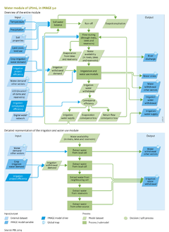
In IMAGE, the hydrological cycle is represented by LPJmL ([[Sitch et al., 2003]]; [[Bondeau et al., 2007]]; [[Gerten et al., 2013]]), which simulates the global hydrological cycle as part of the dynamics of natural vegetation and agricultural production systems. Because LPJmL is linked to IMAGE, there is consistency in the way the [[Carbon cycle and natural vegetation|carbon cycle, natural vegetation]] dynamics, [[Crops and grass|crop growth and production]], [[land-use allocation]] and the water balance can be modelled. | |||
Data on annual [[land cover and land use]] are used as input to LPJmL, including information on the location of irrigated areas and crop types (Figure Flowchart and Input/Output Table at [[Water|Introduction part]]). This affects the amount of water that evaporates and runs off, as well as the amount of water needed for irrigated areas during the (simulated) growing season of crops. Similarly, information on water availability calculated by LPJmL is taken into account in the [[Land-use allocation]] model to identify suitable locations to expand irrigated areas. | |||
Climate is used as input in LPJmL to determine potential evapotranspiration, and the precipitation input to the water balance ([[Gerten et al., 2004]]). The [[Crops and grass]] module, which is also part of LPJmL, calculates irrigation water demand based on crop characteristics, soil moisture and climate. If the amount of water available for irrigation is limited, water stress will occur which leads to reduction of crop yields calculated by the [[Crops and grass|crop and grassland]] model. | |||
===The natural hydrological cycle=== | |||
The Hydrology module in LPJmL consists of a vertical water balance ([[Gerten et al., 2004]]) and a lateral flow component ([[Rost et al., 2008]]) which are run at 0.5 degree resolution in daily time steps (Figure Flowchart). The soil in each grid cell is represented by a two-layer soil column of 0.5 and 1.0 m depth, partly covered with natural vegetation or crops. | |||
The potential evapotranspiration rate in each grid cell depends primarily on net radiation and temperature, and is calculated using the Priestley-Taylor approach ([[Gerten et al., 2004]]). The actual evapotranspiration is calculated as the sum of three components: evaporation of water stored in the canopy (interception), bare soil evaporation and plant transpiration ([[Gerten et al., 2004]]). Water storage in the canopy is a function of vegetation type, leaf area index ({{abbrTemplate|LAI}}) and precipitation amount. Plant transpiration is modelled as the minimum of atmospheric demand and plant water supply. Plant water supply depends on the plant-dependent maximum transpiration rate and relative soil moisture. Soil evaporation occurs in the proportion of land in the grid cell that is not covered by vegetation. It equals potential evaporation when the soil moisture of the upper 20 cm is at field capacity, and declines linearly with relative soil moisture. | |||
Precipitation reaching the soil (throughfall, precipitation minus interception) either accumulates as snow or infiltrates into the soil. Snowmelt is calculated using a simple degree-day method ([[Gerten et al., 2004]]). The soil is parameterised as a bucket model. The status of soil moisture of the two soil layers is updated daily, accounting for throughfall, snowmelt, evapotranspiration, percolation and runoff. Percolation rates for the two soil layers depend on soil type and decline exponentially with soil moisture. Total runoff is calculated as water in excess of field capacity from the two soil layers and water percolating through the second soil layer. The current version of LPJmL has no explicit representation of groundwater recharge, but a groundwater scheme is under development. The daily (subsurface) runoff includes the renewable fraction of groundwater, but without any time delay. | |||
The | All runoff is routed daily through a gridded river network, representing a system of rivers, natural lakes and reservoirs, using a simple routing algorithm ([[Rost et al., 2008]]). Local runoff is added to surface water storage in the cell, and subsequently flows downstream at a constant flow velocity of 1 m s-1 until reaching a lake or reservoir. Water accumulates in lakes and reservoirs, and outflow depends on actual storage relative to the maximum storage capacity (for lakes) and the operational purpose of the reservoir ([[Biemans et al., 2011]]). For man-made reservoirs, see further below ([[Biemans et al., 2011]]) | ||
===Supply and demand for irrigation water=== | |||
Water availability and demand in agriculture is simulated with LPJmL’s irrigation algorithm and an algorithm to simulate the operation of large reservoirs to supply water to irrigated areas ([[Biemans et al., 2013]]). | |||
The irrigation demand submodel (Figure Flowchart) is described in detail by Rost et al. ([[Rost et al., 2008|2008]]). Crop net irrigation demand is defined as the minimum atmospheric evaporative demand and the amount of water needed to fill the soil to field capacity. The irrigation withdrawal demand – the gross demand – is subsequently calculated as the product of the crop irrigation demand and a country-specific irrigation efficiency factor that reflects the type and efficiency of prevailing irrigation systems ([[Rost et al., 2008]]). The efficiency, i.e. the losses of withdrawn water during transport between withdrawal point and irrigated field depends on the type of conveyance system (e.g., open channel or pipeline). Thus, the quantity of water demanded by crops (water consumption) is always less than the quantity withdrawn (water use). | |||
Irrigation water is extracted from the rivers and lakes in the grid cell or a neighbouring grid cell. If these local surface water sources cannot meet the total demand, water is extracted from nearby reservoirs, if available. Finally, water can be supplied from an unlimited source that can be interpreted as non-sustainable groundwater or water imported from another basin. By excluding these water sources in a series of model runs, irrigation water supply and crop production can be attributed to different water sources. | |||
===Large reservoirs=== | |||
Some 50% of global river systems are regulated by dams, most of which are in basins where there is irrigation and economic activity ([[Nilsson et al., 2005]]). The main purpose of approximately one-third of all large reservoirs is irrigation. Thus, in estimating agricultural water use, man-made reservoirs have to be taken into account. | |||
The reservoir operation module in LPJmL ([[Biemans et al., 2011]]) distinguishes three types of reservoirs: reservoirs used primarily for irrigation; reservoirs used primarily for other purposes (e.g., hydropower and flood control) but also for irrigation; and reservoirs not used for irrigation. Each type of reservoir is managed differently. The outflow of irrigation reservoirs follows the temporal pattern of irrigation demand, whereas the other reservoirs are intended to release equal quantities of water throughout the year. Water from irrigation reservoirs is supplied to downstream irrigated areas. | |||
===Water demand in other sectors=== | |||
IMAGE-LPJmL only calculates agricultural water demand internally, and water demand in other sectors is calculated separately. For household and manufacturing sectors, data and algorithms are adopted from the WaterGAP model ([[Alcamo et al., 2003]]). For the electricity sector, a process-based estimation is used based on the study by Davies et al. ([[Davies et al., 2013|2013]]), and Livestock water demand follows from the number of animals estimated in the [[Livestock systems]] model, with the water demand per head adjusted for climate conditions. Domestic demand is a function of population size and per capita income, corrected for the proportion of the population without access to a piped water supply (see Component [[Human development]]). Manufacturing demand is a function of industrial value added, corrected for changes in sector composition, such as the structural change factor used for [[Energy demand]]. | |||
For the electricity sector, a technology-based approach was adopted from the study by Davies et al. ([[Davies et al., 2013|2013]]).The type of power plant (e.g., standard steam cycle, combined steam cycle) determines the demand for cooling capacity. As plants cogenerating heat and power require less cooling capacity, demand is also corrected for these plants. In addition, the type of cooling facility determines the quantity of water required. Once-through cooling systems use large volumes of surface water that are returned almost entirely to the water body from which they were extracted, albeit at an elevated temperature. Wet cooling towers exploit the evaporation heat capacity of water and, thus require much lower water volumes. However, a significant part of the cooling water evaporates during the process and does not return to the original water body. In some regions, cooling ponds are used, where cooling water is pumped and recycled in a closed loop, with water demand somewhere between the once-through and wet tower cooling systems. Finally, dry cooling systems are deployed that use air as a coolant and thus do not require cooling water. Based on data from Davies et al. ([[Davies et al., 2013|2013]]), market share for types of cooling systems – for each power plant type distinguished in [[TIMER model|TIMER]] in each world region – are combined with energy input requirements to obtain the total water demand for the electricity sector. | |||
===Water extractions=== | |||
Water requirements in other sectors are extracted from local surface water, if available (rather than from reservoirs). Meeting the demand from these sectors receives priority over water withdrawal for irrigation. | |||
The current version of IMAGE-LPJmL does not take into account the water needs of ecosystems, or other uses, such as shipping and recreation. However, a new module to calculate environmental flow requirements is under development ([[Pastor et al., 2014]]). This module, which constrains water withdrawals so that a minimum environmental flow is guaranteed, will be used to identify possible areas of conflict between water users. | |||
</div> | |||
{{DisplayFigureTemplate|Baseline figure Water}} | |||
<div class="page_standard"> | |||
===Impact indicators=== | |||
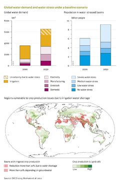
Water stress is often presented as a spatial and temporal average water withdrawal-to-availability ratio at basin or country level. The population living with water stress is estimated by overlaying such a water-stress (or water availability) map with a population density map. These indicators are used to present IMAGE-LPJmL results (for instance, in the [[OECD Environmental Outlook to 2050 (2012) project|OECD Environmental Outlook]], see Figure) but they mask the potential occurrence of water shortages in the short-term or on sub-basin scale. Thus, water stress should also be calculated at higher spatial and temporal resolutions, as can principally be done with LPJmL (see [[Biemans, 2012]]). | |||
The impacts of water stress differ per sector, but the indicators described above do not provide deeper insight into these impacts. In addition to the general water stress indicators, the model also considers production reduction in irrigated agriculture due to limited water availability as an indicator of agricultural water stress ([[Biemans, 2012]]). | |||
</div> | </div> | ||
Revision as of 20:00, 15 November 2018
Parts of Water/Description
| Component is implemented in: |
|
| Related IMAGE components |
| Projects/Applications |
| Key publications |
| References |
Model description of Water
Model description of Water
In IMAGE, the hydrological cycle is represented by LPJmL (Sitch et al., 2003; Bondeau et al., 2007; Gerten et al., 2013), which simulates the global hydrological cycle as part of the dynamics of natural vegetation and agricultural production systems. Because LPJmL is linked to IMAGE, there is consistency in the way the carbon cycle, natural vegetation dynamics, crop growth and production, land-use allocation and the water balance can be modelled.
Data on annual land cover and land use are used as input to LPJmL, including information on the location of irrigated areas and crop types (Figure Flowchart and Input/Output Table at Introduction part). This affects the amount of water that evaporates and runs off, as well as the amount of water needed for irrigated areas during the (simulated) growing season of crops. Similarly, information on water availability calculated by LPJmL is taken into account in the Land-use allocation model to identify suitable locations to expand irrigated areas.
Climate is used as input in LPJmL to determine potential evapotranspiration, and the precipitation input to the water balance (Gerten et al., 2004). The Crops and grass module, which is also part of LPJmL, calculates irrigation water demand based on crop characteristics, soil moisture and climate. If the amount of water available for irrigation is limited, water stress will occur which leads to reduction of crop yields calculated by the crop and grassland model.
The natural hydrological cycle
The Hydrology module in LPJmL consists of a vertical water balance (Gerten et al., 2004) and a lateral flow component (Rost et al., 2008) which are run at 0.5 degree resolution in daily time steps (Figure Flowchart). The soil in each grid cell is represented by a two-layer soil column of 0.5 and 1.0 m depth, partly covered with natural vegetation or crops.
The potential evapotranspiration rate in each grid cell depends primarily on net radiation and temperature, and is calculated using the Priestley-Taylor approach (Gerten et al., 2004). The actual evapotranspiration is calculated as the sum of three components: evaporation of water stored in the canopy (interception), bare soil evaporation and plant transpiration (Gerten et al., 2004). Water storage in the canopy is a function of vegetation type, leaf area index (LAI) and precipitation amount. Plant transpiration is modelled as the minimum of atmospheric demand and plant water supply. Plant water supply depends on the plant-dependent maximum transpiration rate and relative soil moisture. Soil evaporation occurs in the proportion of land in the grid cell that is not covered by vegetation. It equals potential evaporation when the soil moisture of the upper 20 cm is at field capacity, and declines linearly with relative soil moisture.
Precipitation reaching the soil (throughfall, precipitation minus interception) either accumulates as snow or infiltrates into the soil. Snowmelt is calculated using a simple degree-day method (Gerten et al., 2004). The soil is parameterised as a bucket model. The status of soil moisture of the two soil layers is updated daily, accounting for throughfall, snowmelt, evapotranspiration, percolation and runoff. Percolation rates for the two soil layers depend on soil type and decline exponentially with soil moisture. Total runoff is calculated as water in excess of field capacity from the two soil layers and water percolating through the second soil layer. The current version of LPJmL has no explicit representation of groundwater recharge, but a groundwater scheme is under development. The daily (subsurface) runoff includes the renewable fraction of groundwater, but without any time delay.
All runoff is routed daily through a gridded river network, representing a system of rivers, natural lakes and reservoirs, using a simple routing algorithm (Rost et al., 2008). Local runoff is added to surface water storage in the cell, and subsequently flows downstream at a constant flow velocity of 1 m s-1 until reaching a lake or reservoir. Water accumulates in lakes and reservoirs, and outflow depends on actual storage relative to the maximum storage capacity (for lakes) and the operational purpose of the reservoir (Biemans et al., 2011). For man-made reservoirs, see further below (Biemans et al., 2011)
Supply and demand for irrigation water
Water availability and demand in agriculture is simulated with LPJmL’s irrigation algorithm and an algorithm to simulate the operation of large reservoirs to supply water to irrigated areas (Biemans et al., 2013).
The irrigation demand submodel (Figure Flowchart) is described in detail by Rost et al. (2008). Crop net irrigation demand is defined as the minimum atmospheric evaporative demand and the amount of water needed to fill the soil to field capacity. The irrigation withdrawal demand – the gross demand – is subsequently calculated as the product of the crop irrigation demand and a country-specific irrigation efficiency factor that reflects the type and efficiency of prevailing irrigation systems (Rost et al., 2008). The efficiency, i.e. the losses of withdrawn water during transport between withdrawal point and irrigated field depends on the type of conveyance system (e.g., open channel or pipeline). Thus, the quantity of water demanded by crops (water consumption) is always less than the quantity withdrawn (water use).
Irrigation water is extracted from the rivers and lakes in the grid cell or a neighbouring grid cell. If these local surface water sources cannot meet the total demand, water is extracted from nearby reservoirs, if available. Finally, water can be supplied from an unlimited source that can be interpreted as non-sustainable groundwater or water imported from another basin. By excluding these water sources in a series of model runs, irrigation water supply and crop production can be attributed to different water sources.
Large reservoirs
Some 50% of global river systems are regulated by dams, most of which are in basins where there is irrigation and economic activity (Nilsson et al., 2005). The main purpose of approximately one-third of all large reservoirs is irrigation. Thus, in estimating agricultural water use, man-made reservoirs have to be taken into account. The reservoir operation module in LPJmL (Biemans et al., 2011) distinguishes three types of reservoirs: reservoirs used primarily for irrigation; reservoirs used primarily for other purposes (e.g., hydropower and flood control) but also for irrigation; and reservoirs not used for irrigation. Each type of reservoir is managed differently. The outflow of irrigation reservoirs follows the temporal pattern of irrigation demand, whereas the other reservoirs are intended to release equal quantities of water throughout the year. Water from irrigation reservoirs is supplied to downstream irrigated areas.
Water demand in other sectors
IMAGE-LPJmL only calculates agricultural water demand internally, and water demand in other sectors is calculated separately. For household and manufacturing sectors, data and algorithms are adopted from the WaterGAP model (Alcamo et al., 2003). For the electricity sector, a process-based estimation is used based on the study by Davies et al. (2013), and Livestock water demand follows from the number of animals estimated in the Livestock systems model, with the water demand per head adjusted for climate conditions. Domestic demand is a function of population size and per capita income, corrected for the proportion of the population without access to a piped water supply (see Component Human development). Manufacturing demand is a function of industrial value added, corrected for changes in sector composition, such as the structural change factor used for Energy demand.
For the electricity sector, a technology-based approach was adopted from the study by Davies et al. (2013).The type of power plant (e.g., standard steam cycle, combined steam cycle) determines the demand for cooling capacity. As plants cogenerating heat and power require less cooling capacity, demand is also corrected for these plants. In addition, the type of cooling facility determines the quantity of water required. Once-through cooling systems use large volumes of surface water that are returned almost entirely to the water body from which they were extracted, albeit at an elevated temperature. Wet cooling towers exploit the evaporation heat capacity of water and, thus require much lower water volumes. However, a significant part of the cooling water evaporates during the process and does not return to the original water body. In some regions, cooling ponds are used, where cooling water is pumped and recycled in a closed loop, with water demand somewhere between the once-through and wet tower cooling systems. Finally, dry cooling systems are deployed that use air as a coolant and thus do not require cooling water. Based on data from Davies et al. (2013), market share for types of cooling systems – for each power plant type distinguished in TIMER in each world region – are combined with energy input requirements to obtain the total water demand for the electricity sector.
Water extractions
Water requirements in other sectors are extracted from local surface water, if available (rather than from reservoirs). Meeting the demand from these sectors receives priority over water withdrawal for irrigation.
The current version of IMAGE-LPJmL does not take into account the water needs of ecosystems, or other uses, such as shipping and recreation. However, a new module to calculate environmental flow requirements is under development (Pastor et al., 2014). This module, which constrains water withdrawals so that a minimum environmental flow is guaranteed, will be used to identify possible areas of conflict between water users.
Impact indicators
Water stress is often presented as a spatial and temporal average water withdrawal-to-availability ratio at basin or country level. The population living with water stress is estimated by overlaying such a water-stress (or water availability) map with a population density map. These indicators are used to present IMAGE-LPJmL results (for instance, in the OECD Environmental Outlook, see Figure) but they mask the potential occurrence of water shortages in the short-term or on sub-basin scale. Thus, water stress should also be calculated at higher spatial and temporal resolutions, as can principally be done with LPJmL (see Biemans, 2012).
The impacts of water stress differ per sector, but the indicators described above do not provide deeper insight into these impacts. In addition to the general water stress indicators, the model also considers production reduction in irrigated agriculture due to limited water availability as an indicator of agricultural water stress (Biemans, 2012).