Flood risks/Description: Difference between revisions
Jump to navigation
Jump to search
No edit summary |
ArnoBouwman (talk | contribs) No edit summary |
||
| Line 1: | Line 1: | ||
{{ComponentDescriptionTemplate | {{ComponentDescriptionTemplate | ||
|Status=On hold | |Status=On hold | ||
|Reference=Loveland et al., 2000; Van Beek et al., 2011; Wada et al., 2011; Hinkel and Klein, 2009; | |Reference=Loveland et al., 2000; Van Beek et al., 2011; Wada et al., 2011; Hinkel and Klein, 2009; | ||
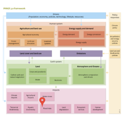
|Description=The purpose of the [[GLOFRIS model]] ([[Winsemius et al., 2012]]; [[Ward et al., 2013]]) is to estimate the effect of land cover and climate change on flood risks in river catchments and coastal areas on a global level. The global flood risks are expressed in the projected number of people affected, annually, and in GDP value. GLOFRIS uses land-cover input from [[IMAGE land use model|IMAGE]] and climate time series, such as the IPCC GCM projections. These input data drive a global hydrological model ([[PCR-GLOBWB model|PCR-GLOBWB]], the computational core of the module). PCR-GLOBWB calculates where and when flooding events may occur, and calculates the inundation extent and depth needed to estimate flood risks. PCR-GLOBWB has features (daily time steps and proper accounting of the relationship between non-linear soil moisture and run-off) that make this model appropriate for simulating flooding events. The spatial resolution currently used by the model is 0.5 x 0.5 degrees (and 5 x 5 minute resolution, currently under development). The different model steps of the main GLOFRIS module are shown in the model flow diagram of GLOFRIS on the right. | |Description===The flood model== | ||
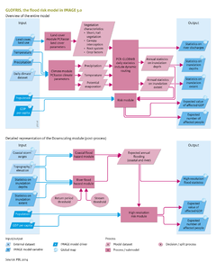
The purpose of the [[GLOFRIS model]] ([[Winsemius et al., 2012]]; [[Ward et al., 2013]]) is to estimate the effect of land cover and climate change on flood risks in river catchments and coastal areas on a global level. The global flood risks are expressed in the projected number of people affected, annually, and in GDP value. GLOFRIS uses land-cover input from [[IMAGE land use model|IMAGE]] and climate time series, such as the IPCC GCM projections. These input data drive a global hydrological model ([[PCR-GLOBWB model|PCR-GLOBWB]], the computational core of the module). PCR-GLOBWB calculates where and when flooding events may occur, and calculates the inundation extent and depth needed to estimate flood risks. PCR-GLOBWB has features (daily time steps and proper accounting of the relationship between non-linear soil moisture and run-off) that make this model appropriate for simulating flooding events. The spatial resolution currently used by the model is 0.5 x 0.5 degrees (and 5 x 5 minute resolution, currently under development). The different model steps of the main GLOFRIS module are shown in the model flow diagram of GLOFRIS on the right. | |||
==Land cover.== | |||
The land-cover map ‘Global Land Cover Characterization’ ([[HasAcronym::GLCC]]) ([[Loveland et al., 2000]]) is the basis of the parameters of the PCR-GLOBWB hydrological model (model flow diagram of GLOFRIS on the right). These parameters express the hydrological characteristics of different land-cover types. IMAGE and PCR-GLOBWB are linked by lookup tables that translate the IMAGE land-cover classification into that of GLCC. | The land-cover map ‘Global Land Cover Characterization’ ([[HasAcronym::GLCC]]) ([[Loveland et al., 2000]]) is the basis of the parameters of the PCR-GLOBWB hydrological model (model flow diagram of GLOFRIS on the right). These parameters express the hydrological characteristics of different land-cover types. IMAGE and PCR-GLOBWB are linked by lookup tables that translate the IMAGE land-cover classification into that of GLCC. | ||
==Flood hazard.== | |||
The hydrological model PCR-GLOBWB ([[Van Beek et al., 2011]]; [[Wada et al., 2011]]) requires data on daily precipitation, potential evaporation and temperature that are consistent with the IMAGE scenario. Daily data are required because that reflects intermonthly and interannual climate variability and its effect on flood risk. | The hydrological model PCR-GLOBWB ([[Van Beek et al., 2011]]; [[Wada et al., 2011]]) requires data on daily precipitation, potential evaporation and temperature that are consistent with the IMAGE scenario. Daily data are required because that reflects intermonthly and interannual climate variability and its effect on flood risk. | ||
The PCR-GLOBWB model includes a routing component on river flooding that estimates inundation fractions and average inundation depths on a time-step basis. These inundation fractions and depths are used to estimate flood risk. GLOFRIS scenarios typically cover a 30-year or longer climatological model run; from this time series, annual extreme values of the inundated fractions and water depths are derived and summarised in an extreme value probability distribution. This probability distribution is subsequently used for annual projections on the damage of flood risk. | The PCR-GLOBWB model includes a routing component on river flooding that estimates inundation fractions and average inundation depths on a time-step basis. These inundation fractions and depths are used to estimate flood risk. GLOFRIS scenarios typically cover a 30-year or longer climatological model run; from this time series, annual extreme values of the inundated fractions and water depths are derived and summarised in an extreme value probability distribution. This probability distribution is subsequently used for annual projections on the damage of flood risk. | ||
==Downscaling== | |||
GLOFRIS estimates flood risk on two scales: that of 0.5 x 0.5 degrees for global analyses and that of 1 x 1 km<sup>2</sup> for specific case studies. On a global scale, the extreme value probability distribution is directly combined with data on population and GDP, using a linear flood level–damage relationship. This means that, for each year of simulation, the most extreme water level and inundated fraction from PCR-GLOBWB is used to calculate the maximum damage (in GDP or population) per grid cell. | GLOFRIS estimates flood risk on two scales: that of 0.5 x 0.5 degrees for global analyses and that of 1 x 1 km<sup>2</sup> for specific case studies. On a global scale, the extreme value probability distribution is directly combined with data on population and GDP, using a linear flood level–damage relationship. This means that, for each year of simulation, the most extreme water level and inundated fraction from PCR-GLOBWB is used to calculate the maximum damage (in GDP or population) per grid cell. | ||
An algorithm is implemented to scale down the 0.5 x 0.5 degree maps of the extent and depth of annual maximum inundation to 1 x 1 km<sup>2</sup>, using a high-resolution digital elevation model. A scale down is needed, because the spatial variability of both flood hazards and flood exposure may be large and are not well represented on the coarser scales of IMAGE and PCR-GLOBWB. Therefore, a more accurate estimation of flood risk is obtained by converting the results to a higher resolution. This downscaling procedure may also include the risk of coastal flooding (Model flow diagram of the downscaling routine on the right). | An algorithm is implemented to scale down the 0.5 x 0.5 degree maps of the extent and depth of annual maximum inundation to 1 x 1 km<sup>2</sup>, using a high-resolution digital elevation model. A scale down is needed, because the spatial variability of both flood hazards and flood exposure may be large and are not well represented on the coarser scales of IMAGE and PCR-GLOBWB. Therefore, a more accurate estimation of flood risk is obtained by converting the results to a higher resolution. This downscaling procedure may also include the risk of coastal flooding (Model flow diagram of the downscaling routine on the right). | ||
For the scaling down in river catchments, annual extreme values of inundation depths and fractions are transformed into bankfull volumes and excess volumes per 0.5 degree cell. The bankfull volume represents the volumetric capacity of a river channel within a particular grid cell and is estimated according to flood volume, associated with a user-defined return period in which flood volumes will not lead to exceeding the bankfull volume (return period threshold in the model flow diagram of the downscaling routine on the right) under current climate and land-cover conditions. The excess bankfull volume for each year is scaled down by estimating a water level from identified river pixels, determined by the user-defined stream threshold (see Model flow diagram of the downscaling routine on the right) that generates a flood volume in the surrounding connected pixels, resulting in the same flood volume, estimated from the 0.5 x 0.5 degree results. The method is therefore mass conservative with respect to the PCR-GLOBWB results on 0.5 degree cells. | For the scaling down in river catchments, annual extreme values of inundation depths and fractions are transformed into bankfull volumes and excess volumes per 0.5 degree cell. The bankfull volume represents the volumetric capacity of a river channel within a particular grid cell and is estimated according to flood volume, associated with a user-defined return period in which flood volumes will not lead to exceeding the bankfull volume (return period threshold in the model flow diagram of the downscaling routine on the right) under current climate and land-cover conditions. The excess bankfull volume for each year is scaled down by estimating a water level from identified river pixels, determined by the user-defined stream threshold (see Model flow diagram of the downscaling routine on the right) that generates a flood volume in the surrounding connected pixels, resulting in the same flood volume, estimated from the 0.5 x 0.5 degree results. The method is therefore mass conservative with respect to the PCR-GLOBWB results on 0.5 degree cells. | ||
==Coastal flood== | |||
Coastal flood hazard maps are established using the [[DIVA model|DIVA database]]. DIVA contains estimates on 1-, 10-, 100- and 1000-year coastal water levels, along a large number of coasts around the world ([[Hinkel and Klein, 2009]]). These coastal flood probabilities are combined with those on river flooding by finding the upstream connected pixels within the high-resolution elevation map that have a lower elevation than the coastal water levels. In this computation it is assumed that, as a wave moves inland, its height will be reduced as the water spreads over the surface, resulting in lower water levels inland than at the coast. | Coastal flood hazard maps are established using the [[DIVA model|DIVA database]]. DIVA contains estimates on 1-, 10-, 100- and 1000-year coastal water levels, along a large number of coasts around the world ([[Hinkel and Klein, 2009]]). These coastal flood probabilities are combined with those on river flooding by finding the upstream connected pixels within the high-resolution elevation map that have a lower elevation than the coastal water levels. In this computation it is assumed that, as a wave moves inland, its height will be reduced as the water spreads over the surface, resulting in lower water levels inland than at the coast. | ||
==Flood risk== | |||
After the high-resolution flood hazard maps have been established, the annual extreme values can be combined to form average annual flood hazard maps and flood risk maps. At this scale, also more local detail can be applied about cropland locations, high-resolution maps on population and GDP or other exposure data of interest to the user. The resulting flood hazard maps can be combined with these high-resolution maps on population and GDP and, if possible, more localised damage models. | After the high-resolution flood hazard maps have been established, the annual extreme values can be combined to form average annual flood hazard maps and flood risk maps. At this scale, also more local detail can be applied about cropland locations, high-resolution maps on population and GDP or other exposure data of interest to the user. The resulting flood hazard maps can be combined with these high-resolution maps on population and GDP and, if possible, more localised damage models. | ||
More information about GLOFRIS, its underlying models and methods, as well as the downscaling module can be found in Winsemius et al. and Ward et al. ([[Winsemius et al., 2012]]; [[Ward et al., 2013]]). | More information about GLOFRIS, its underlying models and methods, as well as the downscaling module can be found in Winsemius et al. and Ward et al. ([[Winsemius et al., 2012]]; [[Ward et al., 2013]]). | ||
}} | }} | ||
Revision as of 10:11, 19 December 2013
Parts of Flood risks/Description
| Component is implemented in: |
|
| Related IMAGE components |
| Models/Databases |
| Key publications |
| References |