Carbon cycle and natural vegetation/Description: Difference between revisions
No edit summary |
No edit summary |
||
| (31 intermediate revisions by 3 users not shown) | |||
| Line 1: | Line 1: | ||
{{ComponentDescriptionTemplate | {{ComponentDescriptionTemplate | ||
| | |Reference=Prentice et al., 2007; Lauk et al., 2012; Klein Goldewijk et al., 2011; | ||
}} | |||
<div class="page_standard"> | |||
===Vegetation types=== | |||
LPJmL is a Dynamic Global Vegetation Model ({{abbrTemplate|DGVM}}) that was developed initially to assess the role of the terrestrial biosphere in the global carbon cycle ([[Prentice et al., 2007]]). DGVMs simulate vegetation distribution and dynamics, using the concept of multiple plant functional types ({{abbrTemplate|PFT}}s) differentiated according to their bioclimatic (e.g. temperature requirement), physiological, morphological, and phenological (e.g. growing season) attributes, and competition for resources (light and water). | |||
To aggregate the vast diversity of plant species worldwide, with respect to major differences relevant to the carbon cycle, [[LPJmL model|LPJmL]] distinguishes eleven natural plant functional types. These include e.g. tropical evergreen trees, temperate deciduous broad-leaved trees and C3 herbaceous plants. Plant dynamics are computed for each PFT present in a grid cell. As IMAGE uses the concept of biomes (natural land cover types), combinations of PFTs in an area/grid cell are translated into a natural land cover (biome) type (see [[Plant functional types and natural land cover types]]). | |||
===Carbon dynamics=== | ===Carbon dynamics=== | ||
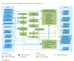
IMAGE-LPJmL covers the carbon cycle processes | IMAGE-LPJmL covers the carbon cycle processes, and tracks all carbon fluxes between the atmosphere and the biosphere. Carbon cycle dynamics of the terrestrial biosphere are computed as carbon uptake and release in plants (photosynthesis, autotrophic respiration), transfer of plant carbon to the soil (shedding of leaves, turnover, mortality) and mineralisation of soil organic matter (heterotrophic respiration; see Figure Flowchart). Because these processes are closely related to weather conditions, they are computed in daily time steps. | ||
The composition of natural vegetation depends on slower processes, such as the inter-annual and inter-seasonal variability in weather conditions and disturbances, such as natural fires. Thus, vegetation dynamics including competition between plant functional types, mortality, turnover, and fire disturbances are computed in annual time steps. | |||
Allocation of newly established biomass is computed in annual time steps for perennial plants (natural grasses, trees) and in daily time steps for annual plants (crops). Allocation to plant organs (represented by a carbon pool for each) distinguishes up to four living plant carbon pools, depending on plant type. For grasses, the model distinguishes carbon pools of leaves and roots only, and for trees, there are two additional woody carbon pools (hardwood and sapwood). For agricultural crops, the pools are categorised as leaves, roots, storage organs, stems, and a mobile reserve pool. | |||
To simulate mineralisation rates of soil organic carbon, the model distinguishes three soil carbon pools for litter, fast soil organic matter (10-year turnover rate) and slow soil organic matter (100-year turnover rate). All carbon from harvested products (crops, grass, biofuels) is assumed to be released to the atmosphere as CO<sub>2</sub> after consumption (food, feed, energy) in the same year. Residues are either left in the fields to enter the litter pool or are removed to subsequently decompose. | |||
During wood harvesting, a proportion of the plant pools is cut down and harvested, as determined in the [[forest management]] model . The waste is left to enter the soil litter pool as dead biomass. Three classes of wood products are distinguished to account for differences in lifespan: | |||
# Pulp and paper has fast turnover rates; | |||
# Timber products, such as furniture, have longer turnover rates ([[Lauk et al., 2012]]); | |||
# Traditional biomass used as an energy source and emitted within the same year. | |||
The IMAGE land-use module (Component [[Agriculture and land use]]) determines annual land-use dynamics, including expansion or abandonment of pastures, cropland and bioenergy plantations, and wood harvested from natural vegetation. | |||
===Model linkage and simulation procedure=== | ===Model linkage and simulation procedure=== | ||
The | The [[LPJmL model]] has multiple links to other IMAGE components and uses IMAGE data on climate, atmospheric CO<sub>2</sub> concentration, land use (including wood demand), and timber use and deforestation (cutting and burning). LPJmL supplies other IMAGE components with information on annual carbon fluxes, net CO<sub>2</sub> exchange between biosphere and atmosphere, size of carbon pools, and natural land cover (biome) classes (see [[Carbon_cycle_and_natural_vegetation|Input/output Table]] at Introduction part ). | ||
LPJmL and IMAGE are linked via an interface and starts in the simulation year of 1970. Before 1970, vegetation and soil carbon pools need to be initialised. This is done by using LPJmL first in a 5000-year spin up to initialise the natural ecosystems and their carbon pools and fluxes, followed by a 390-year spin up, in which agricultural land is gradually expanded based on historical [[HYDE database|HYDE]] land-use data ([[Klein Goldewijk et al., 2011]]). The pool sizes of timber products for 1970 are based on literature estimates ([[Lauk et al., 2012]]). | |||
The linked IMAGE-LPJmL simulations start in 1970 with observed climate, followed by simulated climate from 2015 onwards (Component [[Atmospheric composition and climate]]). As the inter-annual variability in weather conditions is needed for the simulation of vegetation dynamics in IMAGE-LPJmL, smooth annual climate trends from IMAGE are superimposed with inter-annual variability fields, extracted from observed climate over the 1971–2000 period. To avoid repeating climate trends in these 30-year periods, annual anomalies are ordered at random before superimposition. | |||
</div> | |||
Latest revision as of 21:22, 1 November 2021
Parts of Carbon cycle and natural vegetation/Description
| Component is implemented in: |
|
| Related IMAGE components |
| Models/Databases |
| Key publications |
| References |
Model description of Carbon cycle and natural vegetation
Vegetation types
LPJmL is a Dynamic Global Vegetation Model (DGVM) that was developed initially to assess the role of the terrestrial biosphere in the global carbon cycle (Prentice et al., 2007). DGVMs simulate vegetation distribution and dynamics, using the concept of multiple plant functional types (PFTs) differentiated according to their bioclimatic (e.g. temperature requirement), physiological, morphological, and phenological (e.g. growing season) attributes, and competition for resources (light and water).
To aggregate the vast diversity of plant species worldwide, with respect to major differences relevant to the carbon cycle, LPJmL distinguishes eleven natural plant functional types. These include e.g. tropical evergreen trees, temperate deciduous broad-leaved trees and C3 herbaceous plants. Plant dynamics are computed for each PFT present in a grid cell. As IMAGE uses the concept of biomes (natural land cover types), combinations of PFTs in an area/grid cell are translated into a natural land cover (biome) type (see Plant functional types and natural land cover types).
Carbon dynamics
IMAGE-LPJmL covers the carbon cycle processes, and tracks all carbon fluxes between the atmosphere and the biosphere. Carbon cycle dynamics of the terrestrial biosphere are computed as carbon uptake and release in plants (photosynthesis, autotrophic respiration), transfer of plant carbon to the soil (shedding of leaves, turnover, mortality) and mineralisation of soil organic matter (heterotrophic respiration; see Figure Flowchart). Because these processes are closely related to weather conditions, they are computed in daily time steps.
The composition of natural vegetation depends on slower processes, such as the inter-annual and inter-seasonal variability in weather conditions and disturbances, such as natural fires. Thus, vegetation dynamics including competition between plant functional types, mortality, turnover, and fire disturbances are computed in annual time steps.
Allocation of newly established biomass is computed in annual time steps for perennial plants (natural grasses, trees) and in daily time steps for annual plants (crops). Allocation to plant organs (represented by a carbon pool for each) distinguishes up to four living plant carbon pools, depending on plant type. For grasses, the model distinguishes carbon pools of leaves and roots only, and for trees, there are two additional woody carbon pools (hardwood and sapwood). For agricultural crops, the pools are categorised as leaves, roots, storage organs, stems, and a mobile reserve pool.
To simulate mineralisation rates of soil organic carbon, the model distinguishes three soil carbon pools for litter, fast soil organic matter (10-year turnover rate) and slow soil organic matter (100-year turnover rate). All carbon from harvested products (crops, grass, biofuels) is assumed to be released to the atmosphere as CO2 after consumption (food, feed, energy) in the same year. Residues are either left in the fields to enter the litter pool or are removed to subsequently decompose.
During wood harvesting, a proportion of the plant pools is cut down and harvested, as determined in the forest management model . The waste is left to enter the soil litter pool as dead biomass. Three classes of wood products are distinguished to account for differences in lifespan:
- Pulp and paper has fast turnover rates;
- Timber products, such as furniture, have longer turnover rates (Lauk et al., 2012);
- Traditional biomass used as an energy source and emitted within the same year.
The IMAGE land-use module (Component Agriculture and land use) determines annual land-use dynamics, including expansion or abandonment of pastures, cropland and bioenergy plantations, and wood harvested from natural vegetation.
Model linkage and simulation procedure
The LPJmL model has multiple links to other IMAGE components and uses IMAGE data on climate, atmospheric CO2 concentration, land use (including wood demand), and timber use and deforestation (cutting and burning). LPJmL supplies other IMAGE components with information on annual carbon fluxes, net CO2 exchange between biosphere and atmosphere, size of carbon pools, and natural land cover (biome) classes (see Input/output Table at Introduction part ).
LPJmL and IMAGE are linked via an interface and starts in the simulation year of 1970. Before 1970, vegetation and soil carbon pools need to be initialised. This is done by using LPJmL first in a 5000-year spin up to initialise the natural ecosystems and their carbon pools and fluxes, followed by a 390-year spin up, in which agricultural land is gradually expanded based on historical HYDE land-use data (Klein Goldewijk et al., 2011). The pool sizes of timber products for 1970 are based on literature estimates (Lauk et al., 2012).
The linked IMAGE-LPJmL simulations start in 1970 with observed climate, followed by simulated climate from 2015 onwards (Component Atmospheric composition and climate). As the inter-annual variability in weather conditions is needed for the simulation of vegetation dynamics in IMAGE-LPJmL, smooth annual climate trends from IMAGE are superimposed with inter-annual variability fields, extracted from observed climate over the 1971–2000 period. To avoid repeating climate trends in these 30-year periods, annual anomalies are ordered at random before superimposition.