Water/Description: Difference between revisions
< Water
Jump to navigation
Jump to search
No edit summary |
No edit summary |
||
| Line 1: | Line 1: | ||
{{ComponentDescriptionTemplate | {{ComponentDescriptionTemplate | ||
|Status=On hold | |Status=On hold | ||
|Reference=Biemans, 2012; Rost et al., 2008; Gerten et al., 2004; Biemans et al., 2011; Nilsson et al., 2005; Alcamo et al., 2003; Davies et al., 2013; Pastor et al., 2013; | |Reference=Biemans, 2012; Rost et al., 2008; Gerten et al., 2004; Biemans et al., 2011; Nilsson et al., 2005; Alcamo et al., 2003; Davies et al., 2013; Pastor et al., 2013; | ||
|Description=The LPJmL model simulates the global carbon and water balances as part of the dynamics of natural vegetation and agricultural production systems. Because of the coupling of LPJmL to IMAGE, the carbon cycle, natural vegetation, crop production ([[C cycle and natural vegetation dynamics]] and [[Crop and grassland model]]), land-use allocation ([[Forest management]]) and hydrology can be modelled in a consistent way. | |Description=The LPJmL model simulates the global carbon and water balances as part of the dynamics of natural vegetation and agricultural production systems. Because of the coupling of LPJmL to IMAGE, the carbon cycle, natural vegetation, crop production ([[C cycle and natural vegetation dynamics]] and [[Crop and grassland model]]), land-use allocation ([[Forest management]]) and hydrology can be modelled in a consistent way. | ||
==The ‘natural’ hydrological cycle== | ==The ‘natural’ hydrological cycle== | ||
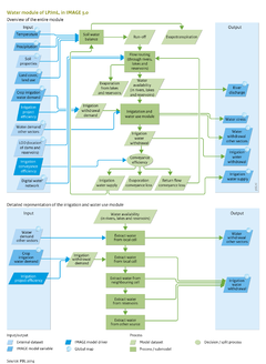
The hydrological module in the LPJmL model consists of a vertical water balance (Gerten et al., 2004) and a lateral flow component ([[Rost et al., 2008]]) (Figure 6.3.1a[[*********]]), which are run at 0.5 degree resolution in time steps of one day. The soil in each grid cell is represented by a two-layer soil column of 0.5 and 1 metre depth, respectively, partly covered with natural vegetation or crops. | The hydrological module in the LPJmL model consists of a vertical water balance (Gerten et al., 2004) and a lateral flow component ([[Rost et al., 2008]]) (Figure 6.3.1a[[*********]]), which are run at 0.5 degree resolution in time steps of one day. The soil in each grid cell is represented by a two-layer soil column of 0.5 and 1 metre depth, respectively, partly covered with natural vegetation or crops. | ||
The potential evaporation rate in each grid cell depends primarily on net radiation and temperature, and is calculated using the Priestley-Taylor approach ([[Gerten et al. 2004]]). The actual evapotranspiration is calculated as the sum of three components: evaporation of intercepted precipitation, bare soil evaporation and plant transpiration. ([[Gerten et al., 2004]]). | The potential evaporation rate in each grid cell depends primarily on net radiation and temperature, and is calculated using the Priestley-Taylor approach ([[Gerten et al., 2004]]). The actual evapotranspiration is calculated as the sum of three components: evaporation of intercepted precipitation, bare soil evaporation and plant transpiration. ([[Gerten et al., 2004]]). | ||
The water storage in the canopy is a function of vegetation type, leaf area index ([[LAI]]) and precipitation amount. Interception evaporation occurs at potential evaporation rate, during the fraction of the daytime that the canopy is wet. | The water storage in the canopy is a function of vegetation type, leaf area index ([[LAI]]) and precipitation amount. Interception evaporation occurs at potential evaporation rate, during the fraction of the daytime that the canopy is wet. | ||
Plant transpiration is modelled as the minimum of atmospheric demand and plant water supply. Plant water supply depends on the plant-dependent maximum transpiration rate and relative soil moisture. Soil evaporation occurs in the fraction of land in the grid cell that is not covered by vegetation. Soil evaporation equals potential evaporation when the soil moisture of the upper 20 cm is at field capacity, and declines linearly with relative soil moisture. | Plant transpiration is modelled as the minimum of atmospheric demand and plant water supply. Plant water supply depends on the plant-dependent maximum transpiration rate and relative soil moisture. Soil evaporation occurs in the fraction of land in the grid cell that is not covered by vegetation. Soil evaporation equals potential evaporation when the soil moisture of the upper 20 cm is at field capacity, and declines linearly with relative soil moisture. | ||
| Line 33: | Line 33: | ||
==Water demand in other sectors== | ==Water demand in other sectors== | ||
The IMAGE-LPJmL model only calculates agricultural water demand internally, hence water demand in other sectors (household, livestock, manufacturing and electricity) is calculated separately. For household and manufacturing sectors data and algorithms are adopted from the WaterGAP model ([[Alcamo et al., 2003]]). For the electricity sector, a process-based estimation is used, based on the study by ([[Davies et al., 2013]]), and livestock demand follows from the number of heads, estimated in the livestock production model (see [[Livestock systems]]), with the water demand per head adjusted for climate conditions. Domestic demand is a function of population size and per-capita income, corrected for the share of the population without access to a piped water supply (see [[Human | The IMAGE-LPJmL model only calculates agricultural water demand internally, hence water demand in other sectors (household, livestock, manufacturing and electricity) is calculated separately. For household and manufacturing sectors data and algorithms are adopted from the WaterGAP model ([[Alcamo et al., 2003]]). For the electricity sector, a process-based estimation is used, based on the study by ([[Davies et al., 2013]]), and livestock demand follows from the number of heads, estimated in the livestock production model (see [[Livestock systems]]), with the water demand per head adjusted for climate conditions. Domestic demand is a function of population size and per-capita income, corrected for the share of the population without access to a piped water supply (see [[Human development]]). Manufacturing demand is a function of industrial value added, corrected for changes in sector composition; for example, the structural change factor also used for energy demand (see Section 4.1.1). For the electricity sector, a technology-based approach was adopted from the study by ([[Davies et al., 2013]]). The type of power plant (e.g. standard steam cycle, combined steam cycle) determines the demand for cooling capacity. Cooling demand is also corrected for cogeneration of heat and power, as those plants require far less cooling capacity. In addition, the type of cooling facility in place determines how much water is required. Once-through cooling systems use large volumes of surface water that are returned almost entirely to the water body that they were extracted from, albeit at an elevated temperature. Wet cooling towers exploit the evaporation heat capacity of water and, hence, require much lower water volumes. However, a significant part of the cooling water evaporates during the process and does not return to the original water body. In some regions, cooling ponds are used, where cooling water is pumped and recycled in a closed loop, with water demand characteristics somewhere in-between the once-through and wet tower cooling systems. Finally, dry cooling systems are deployed that use air as a coolant and, therefore, require no cooling water at all. Based on data from ([[Davies et al., 2013]]), market shares of types of cooling systems – for each power plant type distinguished in TIMER, in each world region – are combined with energy input requirements to arrive at the total water demand for the electricity sector. | ||
In the LPJmL model, the water needed in other sectors is extracted from local surface waters, if available (rather than from reservoirs). Meeting the demand from these sectors receives priority over water withdrawal for irrigation. | In the LPJmL model, the water needed in other sectors is extracted from local surface waters, if available (rather than from reservoirs). Meeting the demand from these sectors receives priority over water withdrawal for irrigation. | ||
| Line 42: | Line 42: | ||
Water stress is often presented as a spatially and temporally averaged water withdrawal-to-availability ratio, typically at basin or country level. The amount of people living under water stress is estimated by overlaying a water-stress map with one of population density. Those indicators are used to present IMAGE-LPJmL results (e.g. in the OECD Environmental Outlook, see Figure 6.3.2[[*******]]) but they mask the potential occurrence of water shortages on a short-term or sub-basin scale. Therefore, water stress should also be calculated at higher spatial and temporal resolutions (see e.g. [[Biemans, 2012]]). | Water stress is often presented as a spatially and temporally averaged water withdrawal-to-availability ratio, typically at basin or country level. The amount of people living under water stress is estimated by overlaying a water-stress map with one of population density. Those indicators are used to present IMAGE-LPJmL results (e.g. in the OECD Environmental Outlook, see Figure 6.3.2[[*******]]) but they mask the potential occurrence of water shortages on a short-term or sub-basin scale. Therefore, water stress should also be calculated at higher spatial and temporal resolutions (see e.g. [[Biemans, 2012]]). | ||
The impacts of water stress differ per sector, but the above described indicators do not provide insight into those impacts. Apart from the general water stress indicators, the model also considers production reductions in irrigated agriculture due to limited water availability as an indicator of agricultural water stress ([[Biemans, 2012]]). | The impacts of water stress differ per sector, but the above described indicators do not provide insight into those impacts. Apart from the general water stress indicators, the model also considers production reductions in irrigated agriculture due to limited water availability as an indicator of agricultural water stress ([[Biemans, 2012]]). | ||
}} | }} | ||
Revision as of 11:15, 10 December 2013
Parts of Water/Description
| Component is implemented in: |
|
| Related IMAGE components |
| Projects/Applications |
| Key publications |
| References |