Carbon cycle and natural vegetation/Description: Difference between revisions
Jump to navigation
Jump to search
No edit summary |
No edit summary |
||
| Line 2: | Line 2: | ||
|Status=On hold | |Status=On hold | ||
|Description===Vegetation types== | |Description===Vegetation types== | ||
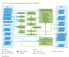
LPJmL is a Dynamic Global Vegetation Model (DGVM), initially developed to assess the role of the terrestrial biosphere in the global carbon cycle (Prentice et al., 2007). DGVMs simulate vegetation distribution and dynamics, using the concept of multiple plant functional types (PFTs) that are differentiated according to their bioclimatic (e.g. temperature requirement), physiological, morphological, and phenological (e.g. growing season) attributes, and that compete for resources (i.e. light and water). In order to aggregate the vast diversity of plant species in the world, with respect to the most important differences for the carbon cycle, LPJmL distinguishes nine PFTs (e.g. tropical evergreen trees, temperate deciduous broad-leaved trees and C3 herbaceous plants). Plant dynamics are computed for each PFT present in a grid cell. Since IMAGE uses the concept of biomes, combinations of PFTs in an area/grid cell are translated into a certain biome type (Appendix, Figure 6.1.2). In the IMAGE framework there is one modification to LPJml, namely the biome ‘ice’, for biomes initially defined as ‘arctic tundra’, and with an average annual temperature of < -2 oC and an annual net primary production (NPP) of < 1 Pg.yr-1 (Appendix, Figure 6.1.2). All carbon pools and fluxes in this biome are set to zero. | LPJmL is a Dynamic Global Vegetation Model ([[hasAcronym::DGVM]]), initially developed to assess the role of the terrestrial biosphere in the global carbon cycle (Prentice et al., 2007). DGVMs simulate vegetation distribution and dynamics, using the concept of multiple plant functional types (PFTs) that are differentiated according to their bioclimatic (e.g. temperature requirement), physiological, morphological, and phenological (e.g. growing season) attributes, and that compete for resources (i.e. light and water). In order to aggregate the vast diversity of plant species in the world, with respect to the most important differences for the carbon cycle, LPJmL distinguishes nine PFTs (e.g. tropical evergreen trees, temperate deciduous broad-leaved trees and C3 herbaceous plants). Plant dynamics are computed for each PFT present in a grid cell. Since IMAGE uses the concept of biomes, combinations of PFTs in an area/grid cell are translated into a certain biome type (Appendix, Figure 6.1.2). In the IMAGE framework there is one modification to LPJml, namely the biome ‘ice’, for biomes initially defined as ‘arctic tundra’, and with an average annual temperature of < -2 oC and an annual net primary production (NPP) of < 1 Pg.yr-1 (Appendix, Figure 6.1.2). All carbon pools and fluxes in this biome are set to zero. | ||
==Carbon dynamics== | ==Carbon dynamics== | ||
| Line 8: | Line 8: | ||
==Model linkage and simulation procedure== | ==Model linkage and simulation procedure== | ||
The technical link between LPJmL and IMAGE is established via an interface and starts in the simulation year of 1970. Before the coupled simulation is started, vegetation and soil carbon pools need to be initialised. This is achieved by using LPJmL first in a 1000-year spin-up in order to initialise the natural ecosystems and their carbon pools and fluxes. This is followed by a 390-year spin-up, in which the agricultural land is gradually expanded based on historical HYDE land-use data (Klein Goldewijk et al., 2011). Timber product pool sizes of 1970 are based on literature estimates (Lauk et al., 2012). The coupled IMAGE-LPJmL simulations start in 1970 with observed climate, followed by simulated climate for the years from 2000 onwards (Section 6.5). As the interannual variability of weather conditions is needed for the simulation of vegetation dynamics in IMAGE-LPJmL, smooth annual climate trends from IMAGE are superimposed by interannual variability fields, extracted from observed climate over the 1971–2000 period. To avoid repeating climate trends within these 30-year periods, annual anomalies are ordered at random before superimposition. | The technical link between LPJmL and IMAGE is established via an interface and starts in the simulation year of 1970. Before the coupled simulation is started, vegetation and soil carbon pools need to be initialised. This is achieved by using LPJmL first in a 1000-year spin-up in order to initialise the natural ecosystems and their carbon pools and fluxes. This is followed by a 390-year spin-up, in which the agricultural land is gradually expanded based on historical HYDE land-use data (Klein Goldewijk et al., 2011). Timber product pool sizes of 1970 are based on literature estimates (Lauk et al., 2012). The coupled IMAGE-LPJmL simulations start in 1970 with observed climate, followed by simulated climate for the years from 2000 onwards (Section 6.5). As the interannual variability of weather conditions is needed for the simulation of vegetation dynamics in IMAGE-LPJmL, smooth annual climate trends from IMAGE are superimposed by interannual variability fields, extracted from observed climate over the 1971–2000 period. To avoid repeating climate trends within these 30-year periods, annual anomalies are ordered at random before superimposition. | ||
}} | }} | ||
Revision as of 16:57, 6 January 2014
Parts of Carbon cycle and natural vegetation/Description
| Component is implemented in: |
|
| Related IMAGE components |
| Models/Databases |
| Key publications |
| References |