IMAGE framework summary/Description: Difference between revisions
Jump to navigation
Jump to search
No edit summary |
No edit summary |
||
| Line 3: | Line 3: | ||
|PageLabel=Detailed description | |PageLabel=Detailed description | ||
|Sequence=2 | |Sequence=2 | ||
|Reference=PBL, 2012; | |||
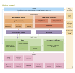
|Description={{DisplayFigureTemplate|Flowchart IF}} | |Description={{DisplayFigureTemplate|Flowchart IF}} | ||
==The IMAGE framework== | ==The IMAGE framework== | ||
| Line 9: | Line 10: | ||
===Projections for driving forces, population and economic development=== | ===Projections for driving forces, population and economic development=== | ||
Key inputs for the model are projections describing direct and indirect drivers of global environmental change ( | Key inputs for the model are projections describing direct and indirect drivers of global environmental change ([[Drivers of framework]]). Most of these drivers (such as technology and lifestyle assumptions) are used as input in various subcomponents of IMAGE (see figure on the right). Clearly, the exogenous assumptions made on these factors need to be consistent. To ensure this, so-called storylines are used, brief stories about how the future may unfold, that can be used to derive internally consistent assumptions for main driving forces. Important categories of scenario drivers include demographic factors, economic development, lifestyle, and technology change. Among these, population and economic development form a special category as they can be dealt with in quantitative sense as exogenous model drivers. Other drivers mostly concern assumptions in different subcomponents of IMAGE, for examplee.g. both the yield assumptions in the crop growth model and the performance of solar power production in the energy model depend on a more generic description of the rate of technology change. | ||
For population, the IMAGE model mostly uses exogenous assumptions (total population per region, household size and urbanization rate). Also the population projections of the PBL GISMO model can be used, which allows, in principle, to also account for feedback of environmental factors (e.g. air pollution and undernourishment) on population growth (see | For population, the IMAGE model mostly uses exogenous assumptions (total population per region, household size and urbanization rate). Also the population projections of the [[PBL]] [[GISMO model]] can be used, which allows, in principle, to also account for feedback of environmental factors (e.g. air pollution and undernourishment) on population growth (see [[Impacts]]). For that purpose, population can be downscaled to the grid level. For economic variables such as [[GDP]], usually also exogenous assumptions are used. In most studies the economic projections are developed by macro-economic models based on the same storylines as the rest of the IMAGE model to ensure consistency. Sector specific economics and household consumption can be derived directly by such models, in addition the latter can be broken down into income categories, reflecting the so-called GINI coefficient (a measure of the disparity in income distribution). | ||
Assumptions for future scenarios start from observed trends in recent decades and this is also the base for the baseline scenario used in the Rio+20 study (PBL 2012)). The global population is based on the UN medium projection and grows to about 9 billion people in 2050, the increase mostly occurring in developing countries | Assumptions for future scenarios start from observed trends in recent decades and this is also the base for the baseline scenario used in the Rio+20 study ([[PBL, 2012]])). The global population is based on the UN medium projection and grows to about 9 billion people in 2050, the increase mostly occurring in developing countries. The economic projection shows that developing countries increasingly dominate the world economy in terms of total GDP. For the [[OECD]] countries, the baseline scenario assumes a long-term economic growth rate of 1-2% per year over the whole scenario period. In the short term, per capita growth rates in Asia and Latin America are much higher, but they start to converge gradually to a long-term growth rates of around 2% per year. Africa, in contrast, shows a later peak in economic growth. | ||
===Human activities in relation to environmental change: the energy and land use system === | ===Human activities in relation to environmental change: the energy and land use system === | ||
Two key areas of human activity play a key role in many environmental and sustainable development issues: 1) energy use and supply ( | Two key areas of human activity play a key role in many environmental and sustainable development issues: 1) energy use and supply ([[Energy supply and demand]]) and 2) food consumption and supply ([[Agriculture and land use]]). Hence, in the IMAGE model, these human activities are the centers of attention. | ||
====Energy supply and demand==== | ====Energy supply and demand==== | ||
For energy use and supply, the IMAGE framework uses a detailed energy system model (The IMage Energy Regional model, TIMER) to describe the long-term dynamics of the energy system; see | For energy use and supply, the IMAGE framework uses a detailed energy system model (The IMage Energy Regional model, [[TIMER model|TIMER]]) to describe the long-term dynamics of the energy system; see [[Energy supply and demand]]. This includes demand for energy services and end-use energy carriers, and the role of fossil fuels versus alternative supply options such as renewables and nuclear power to meet the demands . The model determines the demand for energy services on the basis of primary drivers and assumptions on lifestyle. This demand is fulfilled by final energy carriers, which are, in turn, produced from primary energy sources. Both the mix of final energy carriers and the technologies to produce them are chosen on the basis of their relative costs. Key processes that determine these costs include technology development and resource depletion, but also preferences, fuel trade assumptions and policies play a role. The output of the model demonstrates how energy intensity, fuel costs and competing non-fossil supply technologies develop over time. Implementation of emissions mitigation is generally modeled on the basis of price signals. A carbon tax (used as a generic measure of climate policy) induces additional investments in energy efficiency, in fossil-fuel substitution, bioenergy, nuclear power, solar power, wind power and carbon capture and storage. The energy model is linked to other parts of the IMAGE model via calculated emissions (see further) and demand for bio-energy production (generating input into the land use model). | ||
The model can be used to make detailed projections of energy developments, for instance with and without climate policy. In the Rio+20 baseline scenario, the baseline scenario (without climate policy) projects a 65% increase in energy consumption in the 2010-2050 period, driven by continued population and economic growth. With no fundamental change in current policies, fossil fuels are expected to retain a large market share as their market price is expected, to stay below the alternative fuels for the vast majority of applications. In climate policy scenarios, the inclusion of a carbon price leads to a an increased share for of different technologies and resources, such as carbon-capture and storage, nuclear power and renewables; see Figure 2.4. | The model can be used to make detailed projections of energy developments, for instance with and without climate policy. In the Rio+20 baseline scenario, the baseline scenario (without climate policy) projects a 65% increase in energy consumption in the 2010-2050 period, driven by continued population and economic growth. With no fundamental change in current policies, fossil fuels are expected to retain a large market share as their market price is expected, to stay below the alternative fuels for the vast majority of applications. In climate policy scenarios, the inclusion of a carbon price leads to a an increased share for of different technologies and resources, such as carbon-capture and storage, nuclear power and renewables; see Figure 2.4. | ||
====Food consumption and agriculture==== | ====Food consumption and agriculture==== | ||
Demand for and production of agricultural products are modeled by soft-coupled agro-economic models, mostly MAGNET and IMPACT. With the MAGNET model information can be exchanged in two ways: the IMAGE model supplies the MAGNET model with information on land-supply curves by region (using the IMAGE crop model). And MAGNET provides information on future agricultural production levels and intensity by region, matching regional demands through trade. The MAGNET model assesses the production of agricultural products on the basis of different combinations of primary production factors (land, labour, capital and natural resources) and intermediate production factors. For the livestock sector, IMAGE makes scenario-specific assumptions about the breakdown of livestock production over different systems. A key purpose of the agro-economy model is to determine regional production levels and the associated yields, taking changes in growing conditions into account. In that context, it should be noted that an increase in demand for agricultural production can be met via increased production based on a land expansion (using the regional land supply curves) and/or intensification of land use: increase in yields. | Demand for and production of agricultural products are modeled by soft-coupled agro-economic models, mostly [[MAGNET model|MAGNET]] and [[IMPACT model|IMPACT]]. With the MAGNET model information can be exchanged in two ways: the IMAGE model supplies the MAGNET model with information on land-supply curves by region (using the IMAGE crop model). And MAGNET provides information on future agricultural production levels and intensity by region, matching regional demands through trade. The MAGNET model assesses the production of agricultural products on the basis of different combinations of primary production factors (land, labour, capital and natural resources) and intermediate production factors. For the livestock sector, IMAGE makes scenario-specific assumptions about the breakdown of livestock production over different systems. A key purpose of the agro-economy model is to determine regional production levels and the associated yields, taking changes in growing conditions into account. In that context, it should be noted that an increase in demand for agricultural production can be met via increased production based on a land expansion (using the regional land supply curves) and/or intensification of land use: increase in yields. | ||
All baseline scenarios, including the Rio+20 baseline, project a strong increase in agricultural production, driven by population growth and changes in dietary patterns in line with increasing per capita income. Consistent with the historical trends, most of the increase will be met through on average higher production per hectare (intensification). Still, in the Rio+20 baseline a further slow expansion of the agricultural area in developing countries can be observed, especially for crops and much less for pastures. Alternative scenarios explore ways to mitigate this agricultural expansion, looking into the influence of enhanced yield increase, reduction of post-harvest losses or dietary changes. | All baseline scenarios, including the Rio+20 baseline, project a strong increase in agricultural production, driven by population growth and changes in dietary patterns in line with increasing per capita income. Consistent with the historical trends, most of the increase will be met through on average higher production per hectare (intensification). Still, in the Rio+20 baseline a further slow expansion of the agricultural area in developing countries can be observed, especially for crops and much less for pastures. Alternative scenarios explore ways to mitigate this agricultural expansion, looking into the influence of enhanced yield increase, reduction of post-harvest losses or dietary changes. | ||
| Line 31: | Line 32: | ||
===Interaction between the human system and environmental system: land allocation and emissions=== | ===Interaction between the human system and environmental system: land allocation and emissions=== | ||
There are several ways by which the human system directly influences the earth system. Land allocation and atmospheric emissions form two of the most important factors, others include water extraction, and water and soil pollution. The two main factors are described in IMAGE in separate sub-models. | There are several ways by which the human system directly influences the earth system. Land allocation and atmospheric emissions form two of the most important factors, others include water extraction, and water and soil pollution. The two main factors are described in IMAGE in separate sub-models. | ||
Also, see the background information on [[Downscaling|Downscaling as a tool to link different geographical scales]]. | |||
====Land allocation==== | ====Land allocation==== | ||
| Line 38: | Line 41: | ||
====Emissions==== | ====Emissions==== | ||
Emissions are described in IMAGE as a function of activity levels in the energy system, in industry, in agriculture, and of the assumed abatement actions ( | Emissions are described in IMAGE as a function of activity levels in the energy system, in industry, in agriculture, and of the assumed abatement actions ([[Emissions]]). The model describes the emissions of all major greenhouse gases, and many air pollutants (calibrated to current international emission inventories). In some cases, the calculation of emissions is done using detailed process representation (e.g. emissions from cultivated land and land-cover change) but, in most cases, exogenous emission factors are used. The development of emission factors over time has been estimated based on relevant hypothesis, sometimes assuming constant emission factors, but often assuming that emission factors decrease over time along with economic development (consistent with the so-called environmental Kuznets curve). Emissions factors of greenhouse gases reflect estimates per region, sector and gas from the FAIR model ([[Climate policy]]). | ||
In the Rio+20 baseline, increasing energy and agricultural production levels lead to an increase of associated greenhouse gas emissions. For air pollutants, the emission trends are more diverse: a decrease is projected in high-income countries, as emission factors drop faster than activity levels increase).In most developing country regions, however, increasing energy production is projected to be associated with more air pollution. The model can also be used to design scenarios that are consistent with different climate targets. For reaching the 2oC target, global GHG emissions would need to be reduced by around 50% in 2050. | In the Rio+20 baseline, increasing energy and agricultural production levels lead to an increase of associated greenhouse gas emissions. For air pollutants, the emission trends are more diverse: a decrease is projected in high-income countries, as emission factors drop faster than activity levels increase). In most developing country regions, however, increasing energy production is projected to be associated with more air pollution. The model can also be used to design scenarios that are consistent with different climate targets. For reaching the 2oC target, global [[GHG]] emissions would need to be reduced by around 50% in 2050. | ||
===The earth system=== | ===The earth system=== | ||
| Line 54: | Line 57: | ||
====Atmospheric composition and climate change==== | ====Atmospheric composition and climate change==== | ||
Data on emissions of greenhouse gases and air pollutants are used in IMAGE to calculate changes in concentrations of greenhouse gases, ozone precursors and species involved in aerosol formation at a global scale ( | Data on emissions of greenhouse gases and air pollutants are used in IMAGE to calculate changes in concentrations of greenhouse gases, ozone precursors and species involved in aerosol formation at a global scale ([[Atmospheric composition and climate]]). Climatic change is calculated as global mean temperature changes using a slightly adapted version of the [[MAGICC]]6 climate model. Climatic change does not manifest itself uniformly over the globe, and patterns of temperature and precipitation are uncertain and differ between complex climate models. Therefore, changes in temperature and precipitation in each 0.5 x 0.5 degree grid cell are derived from the global mean temperature using a pattern-scaling approach. The model accounts for important feedback mechanisms related to changing climate, notably growth characteristics in the crop model, carbon dioxide concentrations (carbon fertilization) and land cover (biome types). | ||
In the Rio+20 baseline, increasing fossil fuel use leads to increasing GHG emissions and air pollution levels. For the 2010–2050 period, GHG emissions are projected to increase by about 60%. As a result global temperature is expected to increase to around 4°C above pre-industrial levels by 2100, most likely passing the 2°C level before 2050; see Figure 2.7. | In the Rio+20 baseline, increasing fossil fuel use leads to increasing [[GHG]] emissions and air pollution levels. For the 2010–2050 period, GHG emissions are projected to increase by about 60%. As a result global temperature is expected to increase to around 4°C above pre-industrial levels by 2100, most likely passing the 2°C level before 2050; see Figure 2.7. | ||
====Water==== | ====Water==== | ||
The LPJmL model used for a description of vegetation and carbon cycle also includes a global hydrological model ( | The [[LPJmL model]] used for a description of vegetation and carbon cycle also includes a global hydrological model ([[Hydrological cycle]]). With this coupled hydrological model, IMAGE scenarios now also capture future changes in water availability, agricultural water use and water shortage.. Water demand for irrigated agriculture is calculated inLPJmL, based on requirements for evapotranspiration for the crop types grown on irrigated land. Water demand for other sectors (households, manufacturing, electricity and livestock) is currently adopted from exogenous scenarios. The most frequently used are WaterGap projections of the University of Kassel, adjusted to remain consistent with projections for households, livestock numbers, industrial value added, and for thermal electricity production as projected with IMAGE-TIMER. | ||
The increases projected in agricultural , energy and industry production households lead to an increasing demand for water. At the same time, climate change also impacts the water cycle. While overall climate change is projected to lead to more precipitation, geographical patterns show changes to both dryer and wetter gridcells. As a result, the water balance improves in some regions, while it deteriorates in other regions. The pattern of these changes is very uncertain. In combination with increased demand, however, the number of people confronted with serious water stress is projected to increase significantly. | The increases projected in agricultural , energy and industry production households lead to an increasing demand for water. At the same time, climate change also impacts the water cycle. While overall climate change is projected to lead to more precipitation, geographical patterns show changes to both dryer and wetter gridcells. As a result, the water balance improves in some regions, while it deteriorates in other regions. The pattern of these changes is very uncertain. In combination with increased demand, however, the number of people confronted with serious water stress is projected to increase significantly. | ||
| Line 65: | Line 68: | ||
====Biodiversity loss==== | ====Biodiversity loss==== | ||
Biodiversity loss is described in the impact model GLOBIO in the form of calculated changes in MSA (mean species abundance). The MSA indicator maps the effect of a suite of direct and indirect drivers of biodiversity loss provided by IMAGE. GLOBIO 3 takes into account the impacts of climate, land-use change, ecosystem fragmentation, expansion of infrastructure, disturbance of habitats, and acid and reactive nitrogen deposition ( | Biodiversity loss is described in the impact model [[GLOBIO model|GLOBIO]] in the form of calculated changes in MSA (mean species abundance). The MSA indicator maps the effect of a suite of direct and indirect drivers of biodiversity loss provided by IMAGE. GLOBIO 3 takes into account the impacts of climate, land-use change, ecosystem fragmentation, expansion of infrastructure, disturbance of habitats, and acid and reactive nitrogen deposition ([[Terrestrial biodiversity]]). Their compound effect on biodiversity is computed using the GLOBIO3 model for terrestrial ecosystems. As the IMAGE and the GLOBIO3 models are spatially explicit, the impacts on MSA can be analysed by region, main biome and pressure factor. Recently, a similar model was developed to map biodiversity in fresh water; see [[Aquatic biodiversity]]. | ||
For biodiversity, a further decline is projected in the Rio+20 baseline at an almost unchanged rate as in the past century. While historically, habitat loss has been the most important driver of biodiversity loss, in the future decades climate change, forestry and infrastructure expansion are projected to become the more important pressure factors. | For biodiversity, a further decline is projected in the Rio+20 baseline at an almost unchanged rate as in the past century. While historically, habitat loss has been the most important driver of biodiversity loss, in the future decades climate change, forestry and infrastructure expansion are projected to become the more important pressure factors. | ||
====Human development==== | ====Human development==== | ||
Global environmental change impacts human development in many ways. Via the link to the GISMO model, the IMAGE framework describes impacts on human health, and the achievement of human development goals such as the MDGs. The health model describes the burden of disease per gender and age ( | Global environmental change impacts human development in many ways. Via the link to the [[GISMO model]], the IMAGE framework describes impacts on human health, and the achievement of human development goals such as the [[MDG|MDGs]]. The health model describes the burden of disease per gender and age ([[Human development]]). The GISMO model allows to describe health impacts from communicable diseases, but also from air pollution and undernourishment, and the interactions between these factors. The model is thus able to put the impacts of global environmental change factors in perspective of other factors determining human health. | ||
Hunger, defined as the proportion of the population with food consumption below the minimum dietary energy requirement, is determined using an assumed distribution of food intake over individuals on the basis of the mean food availability per capita (from other parts of IMAGE) and a coefficient of variation. Water supply levels and sanitation were modelled separately for urban and rural populations by applying regressions based on available data for 1990 and 2000. The explanatory variables include GDP per capita, urbanisation rate and population density. | Hunger, defined as the proportion of the population with food consumption below the minimum dietary energy requirement, is determined using an assumed distribution of food intake over individuals on the basis of the mean food availability per capita (from other parts of IMAGE) and a coefficient of variation. Water supply levels and sanitation were modelled separately for urban and rural populations by applying regressions based on available data for 1990 and 2000. The explanatory variables include GDP per capita, urbanisation rate and population density. | ||
| Line 77: | Line 80: | ||
====Other impacts==== | ====Other impacts==== | ||
Other impacts calculated by the IMAGE framework are not described here, including flood risks ( | Other impacts calculated by the IMAGE framework are not described here, including flood risks ([[Flood risks]]), land degradation ([[Soil degradation]]) and ecological goods and services ([[Ecosystem goods and services]]). | ||
}} | }} | ||
Revision as of 11:48, 11 December 2013
| Projects/Applications |
| Relevant overviews |
| Key publications |