IMAGE framework summary/Earth system: Difference between revisions
Jump to navigation
Jump to search
m (Copied from IMAGE framework summary/Drivers) |
No edit summary |
||
| Line 1: | Line 1: | ||
{{FrameworkSummaryPartTemplate | {{FrameworkSummaryPartTemplate | ||
|PageLabel= | |PageLabel=Interaction | ||
|Sequence= | |Sequence=5 | ||
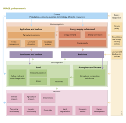
|Description=<h2> | |Description=<h2>Interaction between the Human system and the Earth system</h2> | ||
*land cover/land use | |||
*emissions | |||
The Human system influences the Earth system in various ways, such as land use and atmospheric emissions, but also water extraction, and water and soil pollution. The representation of key factors of land use and atmospheric emissions in the IMAGE model are discussed below. | |||
Land cover and land use | |||
Using demand for agricultural products, including food, feed and bioenergy, the Land-use allocation model locates production areas on a 5 x 5 minute grid (Section 4.2.3). A region-specific regression based suitability assessment and an iterative allocation procedure are used. Alternatively, the land-use model can also integrate CLUMondo (using a more complex allocation procedure). In most regions, the main determinants of suitability for agricultural expansion are population density, accessibility, topography, and agricultural productivity. In the model, suitability is used in combination with regional preferences for different types of production systems (determined from historical calibration) to allocate land use to the grid. In addition, the IMAGE land use and land cover module (Section 5.1) collects and combines information from the agricultural system and the Earth system to provide maps of land-use and land-cover parameters, including fertiliser input, livestock densities, rain-fed and irrigated crop fractions, bioenergy crops, and forest management. | |||
Example: In most baseline scenarios, increased agricultural production in tropical regions leads to loss of natural ecosystems and associated biodiversity loss. Most expansion is projected to occur in highly productive ecosystems close to agricultural areas, including tropical forests and woodland, and other high nature value savannah and grassland areas. The agricultural area is contracting in temperate zones and the grid cells least suitable for production potential are abandoned. The resulting changes in land use are depicted in Figure 2.6. | |||
Figure 2.6: Land cover and land use in 2045 (see also Section 4.2.3) 059X_img13 | |||
Emissions | |||
In IMAGE, emissions are described as a function of activity levels in the energy system, in industry, in agriculture and land-cover and land-use change, and they are also influenced by assumed abatement actions (Section 5.2). The model describes emissions of major greenhouse gases, and many air pollutants, calibrated to current international emission inventories. In some cases, the emission calculation uses detailed process representation on a grid (e.g., emissions from cultivated land and land-cover change) but in most cases, exogenous emission factors are used. Change in emission factors over time is estimated according to the storyline, sometimes assuming constant emission factors, but often assuming emission factors decrease over time along with economic development (consistent with the environmental Kuznets curve). Abatement of greenhouse gas emissions reflects estimates per region, sector and gas often optimised in the FAIR model (Section 8.1). | |||
Example: In the Rio+20 baseline, increasing energy and agricultural production levels lead to an increase of associated greenhouse gas emissions (Figure 2.6). For air pollutants, the emission trends are more diverse. A decrease is projected in high-income countries, as emission factors drop faster than activity levels increase. However, in most developing country regions, increasing energy production is projected to be associated with more air pollution. In the policy scenarios, the target to keep global mean temperature change below 2 °C requires global greenhouse gas emissions to be reduced by about 50% in 2050. This is achieved in the model by structural changes in the energy system and by changes in emission and abatement factors. | |||
Figure 2.7: Changes in emissions under baseline and sustainability scenarios to meet the 2 °C target 013x_img13 | |||
Box 2.2: Downscaling as a tool to link different geographical scales | |||
IMAGE socio-economic modelling is done on the scale of 26 world regions. However, some applications and users of IMAGE output need more detailed information. For this purpose, tools have been developed to downscale information on population, income, energy use and emissions to a 0.5 x 0.5 grid level (Van Vuuren et al., 2007b) and to 5 x 5 minute grid for population and income. Information from the Earth system is available at 0.5 degree or 5 minute resolution. | |||
</BlockQuote> | </BlockQuote> | ||
{{DisplayFigureLeftOptimalTemplate|Figure1 IF}} | {{DisplayFigureLeftOptimalTemplate|Figure1 IF}} | ||
}} | }} | ||
Revision as of 19:52, 9 May 2014
| Projects/Applications |
| Relevant overviews |
| Key publications |
| References |