Crops and grass/Description
Parts of Crops and grass/Description
| Component is implemented in: |
|
| Related IMAGE components |
| Projects/Applications |
| Key publications |
| References |
Model description of Crops and grass
The LPJmL model is a global dynamic vegetation, agriculture and water balance model. The agriculture modules are intrinsically linked to natural vegetation via the carbon and water cycles and follow the same basic process-based modelling approaches, plus additional process representation (management) where needed.
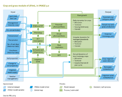
Crop productivity is computed following the same representation of photosynthesis, maintenance and growth respiration as for natural vegetation (see Figure Flowchart Carbon cycle and natural vegetation), but with additional mechanisms for phenological development, allocation of photosynthesis to crop components (leaves, roots, storage organ, mobile pool/stem), and management (Figure Flowchart), which can greatly affect crop productivity and food supply.
In aggregating plant species to classes, the 12 crops currently implemented in LPJmL (Bondeau et al., 2007; Lapola et al., 2009) represent a broader group of crops, referred to as crop functional types (see Crop types in LPJmL). Grassland management can be represented in various ways including regular moving, grazing with different livestock intensities or rotation grazing (Rolinski et al., 2018). The standard setting used in IMAGE 3.2 for pasture is monthly mowing while extensive grasslands are modelled as natural grasslands.
For the cultivation of bioenergy plants, such as short-rotation tree plantations and switch grass, three additional functional types have been introduced: temperate short-rotation coppice trees (e.g., willow); tropical short-rotation coppice trees (e.g., eucalyptus); and Miscanthus (Beringer et al., 2011).
Climate-related management is included in the model endogenously to take account of smart farmer behaviour in long-term simulations. Sowing dates are calculated as a function of farmers’ climate experience (Waha et al., 2012), and also selection of crop varieties (Bondeau et al., 2007).
Individual crops and grass are assumed to be cultivated on separate fields, and thus simulated with separate water balances, but soil properties are averaged in fallow periods to account for crop rotations. All crops in one grid cell are simulated in parallel, both irrigated and non-irrigated crops.
Irrigation modules are constrained by available water from surface water bodies and reservoirs (see Component Water), or assume unconstrained availability of irrigation water (scenario setting) to account for prevalent use of (fossil) groundwater.
To compensate for the absence of an explicit representation of nutrient cycles and other management options that may affect productivity (e.g., pest control, soil preparation), LPJmL can account for management intensity levels, and can be calibrated to reproduce actual FAO yields (Fader et al., 2010). However, given the complex interaction with the Land-use allocation model, LPJmL simulates crop yields without nutrient constraints (potential water-limited yields) in the link with IMAGE. Actual yields are derived by IMAGE by combining potential yields from LPJmL with a management factor that can change over time (see Component Agricultural economy). As input for the IMAGE land-use components (Component Agriculture and land use), LPJmL calculates productivity of each crop in each grid cell under rain-fed and irrigated conditions.
The crop and grassland component is embedded in the dynamic global vegetation, agriculture and water balance model LPJmL, and thus carbon and water dynamics (Components Carbon cycle and natural vegetation and Water, respectively) consistently account for dynamics in agricultural productivity and land-use change.