IMAGE framework summary/Earth system: Difference between revisions
No edit summary |
Dafnomilii (talk | contribs) mNo edit summary |
||
| (33 intermediate revisions by 2 users not shown) | |||
| Line 1: | Line 1: | ||
{{FrameworkSummaryPartTemplate | {{FrameworkSummaryPartTemplate | ||
|PageLabel= | |PageLabel=Earth system | ||
|Sequence= | |Sequence=6 | ||
| | |Reference=Müller et al., 2016b | ||
}} | |||
<div class="page_standard"> | |||
<h2>Carbon cycle and natural vegetation</h2> | |||
In IMAGE 3.0, the terrestrial carbon cycle and natural vegetation dynamics (Component Carbon cycle and natural vegetation) are modelled with [[LPJmL model|LPJmL]]. This model is used to determine productivity at grid cell level for natural ecosystems and crops on the basis of plant and crop functional types. Key inputs to determine productivity include climate conditions, soil types and assumed technology/ management levels. The model iterates with the agricultural production components as it provides input on potential productivity, while land used for agriculture and forestry is a key input. Changes in land cover, land use and climate at grid cell level have consequences for the carbon cycle, and for crop and grass productivity. | |||
<BlockQuote> | <BlockQuote> | ||
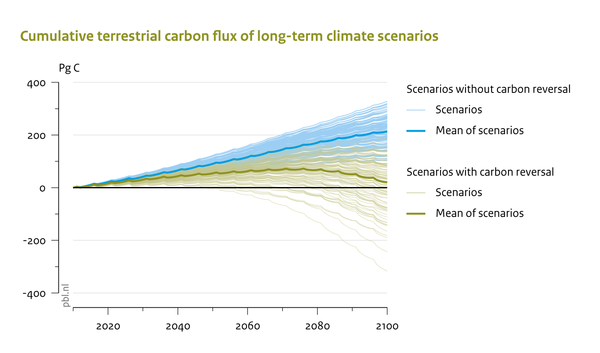
Example: | Example: Food consumption trends lead to net expansion of agricultural land, and thus to net loss of forest (mainly tropical forests). This results in net deforestation emissions as a result of human activities. After 2050, most IMAGE scenarios expect the net anthropogenic emissions from land-use change to decline further and to result in a small net uptake (as a result of demographic trends leading to a decline in land-use for food production). However, the terrestrial vegetation as a whole, which has been a large sink during the last decades, could become a CO<sub>2</sub> source as a result of climate change (the figure below). This could lead to a rapid increase in atmospheric CO<sub>2</sub> concentration, given continued emissions from the energy system. | ||
</BlockQuote> | </BlockQuote> | ||
{{DisplayFigureLeftOptimalTemplate|Baseline figure Carbon cycle and natural vegetation}} | |||
}} | ===Water=== | ||
The LPJmL model used for vegetation and carbon cycle also includes a global hydrology model (Component Water). With this linked hydrology model, IMAGE scenarios capture future changes in irrigated areas, water availability, agricultural water demand and water stress. | |||
Water demand for irrigated agriculture is calculated in LPJmL, based on requirements for evapotranspiration for the crop types grown on irrigated land. For other sectors (households, manufacturing, electricity and livestock), water demand is calculated based on population, economic growth, industrial value added, and electricity production as projected with IMAGE-TIMER. | |||
<BlockQuote> | |||
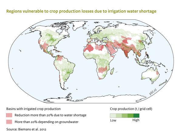
Example: Projected increases in agriculture, energy and industry production, and population lead to increased water demand. Climate change also impacts the water cycle. While overall climate change is projected to lead to more precipitation, geographical patterns show changes to drier and to wetter local climates. In addition, increasing temperature leads to more evapotranspiration. As a result, the water balance improves in some regions and deteriorates in other regions, and the pattern of these changes is very uncertain. In combination with increased demand, the areas confronted with crop production losses are projected to increase significantly as shown in the figure below for a similar scenario. | |||
</BlockQuote> | |||
{{DisplayFigureLeftOptimalTemplate|Baseline figure Water II}} | |||
===Nutrients=== | |||
The Global Nutrient model describes the fate of nitrogen (N) and phosphorus (P) emerging from concentrated point sources, such as human settlements, and from dispersed or non-point sources, such as agricultural and natural land (Component [[Nutrients]]). The nutrient surplus eventually enters coastal water bodies via rivers and lakes. Key drivers that determine nutrient emissions include agricultural production with fertiliser application, and urban and rural populations, and their sanitation systems and level of wastewater treatment. For example, the model calculates the soil nitrogen balance from the total set of inputs and outputs. Inputs include biological nitrogen fixation, atmospheric nitrogen deposition, and application of synthetic nitrogen fertiliser and animal manure. Outputs include nitrogen removal from the field by crop harvesting, grass-cutting and grazing. The nutrient outflow from the soil combined with emissions from point sources and direct atmospheric deposition determine the loading of nutrients to surface water. | |||
<BlockQuote> | |||
Example: In the Rio+20 scenario, further increase in the global population and growth of agricultural production add to pressures on the nutrient cycle. While increasing wastewater treatment and improved agricultural practices mitigate some of the increased nutrient loading, these processes are insufficient to offset increased fertiliser application to sustain intense agriculture. This leads to a significant further imbalance in nitrogen and phosphorus cycles, with consequences for water quality in rivers, lakes and coastal seas. | |||
</BlockQuote> | |||
===Atmospheric composition and climate change=== | |||
Calculated emissions of greenhouse gases and air pollutants are used in IMAGE to derive changes in concentrations of greenhouse gases, ozone precursors and species involved in aerosol formation on a global scale (Component [[Atmospheric composition and climate]]). Climatic change is calculated as global mean temperature change using a slightly adapted version of the [[MAGICC model|MAGICC6.0]] climate model. Climatic change does not manifest uniformly over the globe. The patterns of temperature and precipitation are uncertain and differ between complex climate models. The changes in temperature and precipitation in each 0.5 x 0.5 degrees grid cell are derived from the global mean temperature using a pattern-scaling approach. The model accounts for feedback mechanisms related to changing climate, notably growth characteristics in the crop model, carbon dioxide concentrations (carbon fertilisation) and land cover ([[Land cover types|biome types]]). | |||
<BlockQuote> | |||
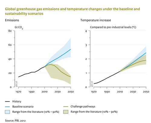
Example: In the Rio+20 baseline, greenhouse gas emissions are projected to increase by about 60% in the 2010-2050 period. As a result, global temperature is expected to increase by around 4 °C above pre-industrial levels by 2100 without climate policy, and most likely exceeding 2 °C before 2050 (the figure below). Rapid emission reductions, however, could limit temperature increase, most likely, to less than 2 °C. | |||
</BlockQuote> | |||
{{DisplayFigureLeftOptimalTemplate|Figure4 IMAGE framework summary}} | |||
</div> | |||
Latest revision as of 15:48, 21 October 2021
| Projects/Applications |
| Relevant overviews |
| Key publications |
| References |
Carbon cycle and natural vegetation
In IMAGE 3.0, the terrestrial carbon cycle and natural vegetation dynamics (Component Carbon cycle and natural vegetation) are modelled with LPJmL. This model is used to determine productivity at grid cell level for natural ecosystems and crops on the basis of plant and crop functional types. Key inputs to determine productivity include climate conditions, soil types and assumed technology/ management levels. The model iterates with the agricultural production components as it provides input on potential productivity, while land used for agriculture and forestry is a key input. Changes in land cover, land use and climate at grid cell level have consequences for the carbon cycle, and for crop and grass productivity.
Example: Food consumption trends lead to net expansion of agricultural land, and thus to net loss of forest (mainly tropical forests). This results in net deforestation emissions as a result of human activities. After 2050, most IMAGE scenarios expect the net anthropogenic emissions from land-use change to decline further and to result in a small net uptake (as a result of demographic trends leading to a decline in land-use for food production). However, the terrestrial vegetation as a whole, which has been a large sink during the last decades, could become a CO2 source as a result of climate change (the figure below). This could lead to a rapid increase in atmospheric CO2 concentration, given continued emissions from the energy system.
Water
The LPJmL model used for vegetation and carbon cycle also includes a global hydrology model (Component Water). With this linked hydrology model, IMAGE scenarios capture future changes in irrigated areas, water availability, agricultural water demand and water stress. Water demand for irrigated agriculture is calculated in LPJmL, based on requirements for evapotranspiration for the crop types grown on irrigated land. For other sectors (households, manufacturing, electricity and livestock), water demand is calculated based on population, economic growth, industrial value added, and electricity production as projected with IMAGE-TIMER.
Example: Projected increases in agriculture, energy and industry production, and population lead to increased water demand. Climate change also impacts the water cycle. While overall climate change is projected to lead to more precipitation, geographical patterns show changes to drier and to wetter local climates. In addition, increasing temperature leads to more evapotranspiration. As a result, the water balance improves in some regions and deteriorates in other regions, and the pattern of these changes is very uncertain. In combination with increased demand, the areas confronted with crop production losses are projected to increase significantly as shown in the figure below for a similar scenario.
Nutrients
The Global Nutrient model describes the fate of nitrogen (N) and phosphorus (P) emerging from concentrated point sources, such as human settlements, and from dispersed or non-point sources, such as agricultural and natural land (Component Nutrients). The nutrient surplus eventually enters coastal water bodies via rivers and lakes. Key drivers that determine nutrient emissions include agricultural production with fertiliser application, and urban and rural populations, and their sanitation systems and level of wastewater treatment. For example, the model calculates the soil nitrogen balance from the total set of inputs and outputs. Inputs include biological nitrogen fixation, atmospheric nitrogen deposition, and application of synthetic nitrogen fertiliser and animal manure. Outputs include nitrogen removal from the field by crop harvesting, grass-cutting and grazing. The nutrient outflow from the soil combined with emissions from point sources and direct atmospheric deposition determine the loading of nutrients to surface water.
Example: In the Rio+20 scenario, further increase in the global population and growth of agricultural production add to pressures on the nutrient cycle. While increasing wastewater treatment and improved agricultural practices mitigate some of the increased nutrient loading, these processes are insufficient to offset increased fertiliser application to sustain intense agriculture. This leads to a significant further imbalance in nitrogen and phosphorus cycles, with consequences for water quality in rivers, lakes and coastal seas.
Atmospheric composition and climate change
Calculated emissions of greenhouse gases and air pollutants are used in IMAGE to derive changes in concentrations of greenhouse gases, ozone precursors and species involved in aerosol formation on a global scale (Component Atmospheric composition and climate). Climatic change is calculated as global mean temperature change using a slightly adapted version of the MAGICC6.0 climate model. Climatic change does not manifest uniformly over the globe. The patterns of temperature and precipitation are uncertain and differ between complex climate models. The changes in temperature and precipitation in each 0.5 x 0.5 degrees grid cell are derived from the global mean temperature using a pattern-scaling approach. The model accounts for feedback mechanisms related to changing climate, notably growth characteristics in the crop model, carbon dioxide concentrations (carbon fertilisation) and land cover (biome types).
Example: In the Rio+20 baseline, greenhouse gas emissions are projected to increase by about 60% in the 2010-2050 period. As a result, global temperature is expected to increase by around 4 °C above pre-industrial levels by 2100 without climate policy, and most likely exceeding 2 °C before 2050 (the figure below). Rapid emission reductions, however, could limit temperature increase, most likely, to less than 2 °C.