IMAGE framework/A brief history of IMAGE: Difference between revisions
Jump to navigation
Jump to search
(Created page with "{{FrameworkIntroductionTemplate}}") |
No edit summary |
||
| Line 1: | Line 1: | ||
{{FrameworkIntroductionTemplate}} | {{FrameworkIntroductionTemplate | ||
|Overview=Rotmans, 1990 | |||
|Reference=Alcamo, 1994; Rotmans, 1990; Alcamo et al., 1998; IMAGE-team, 2001; Bouwman et al., 2006; | |||
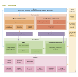
|Description=The IMAGE version 3.0 presented here is the most recent, operational incarnation of the model framework developed out of a suite of earlier versions, going back to the late eighties and published in a series of books. | |||
===IMAGE 1=== | |||
The IMAGE model version 1.0 ([[Rotmans, 1990]]) was developed as a single region, integrated global model to explore the interactions between human activities and future climate change. At the time, IMAGE 1.0 was among the pioneering examples of Integrated Assessment Models addressing climate change. As such, it played an important role in raising awareness of consequences of long-term human development. In the absence of regional or spatially explicit algorithms, the model operated on trends in global total or average parameters, e.g. world population and averaged emission factors per unit of activity. | |||
===IMAGE 2=== | |||
As a result of a major development investment in the nineties, a quite different generation of IMAGE came into operation, jointly referred to as IMAGE 2. The first version, IMAGE 2.0, presented several key aspects retained to date: regional drivers of global change and gridded, process-oriented modeling of the terrestrial biosphere, land-cover and land-use ([[Alcamo, 1994]]). IMAGE 2.0 consisted of three main subsystems: the 13-region Energy-Industry System ([[EIS]]), the Terrestrial Environment System (TES) operating at 0.5x0.5 degrees grid-scale and the Atmosphere-Ocean System ([[AOS]]) to compute the resulting changes in the composition of the atmosphere leading to climate change. Further refinements and extensions were implemented in IMAGE 2.1 ([[Alcamo et al., 1998]]) with the primary aim to enhance the model’s performance and broaden its applicability . The latter was demonstrated convincingly with IMAGE 2.2 contributing to the development and publication of the IPCC Special Report on Emissions Scenarios ([[IMAGE-team, 2001]]). Among others, in IMAGE 2.2 the earlier zonal-mean climate-ocean model was replaced by a combination of the MAGICC climate model and the Bern ocean model. In the new approach, the resulting global average temperature and precipitation changes were scaled using temperature and precipitation patterns generated by complex coupled Global Circulation Models ([[GCM|GCMs]]) to provide spatially explicit climate impacts and feedback. On the economy–energy side, the TIMER energy model replaced the earlier EIS, also improving the linkage with the macro-economic model Worldscan . | |||
===IMAGE 2.4=== | |||
After the release of IMAGE 2.2 at the time of publication of the [[IPCC]]-[[SRES]] report, it was decided to invest in further development of IMAGE, aiming at a next generation, IMAGE 3, and to pursue that with a network strategy, in partnerships with national and international institutes and universities, rather than primarily in-house. IMAGE 2.4 ([[Bouwman et al., 2006]]) marked several major steps towards achieving the ambitions of IMAGE 3. Important changes include the close coupling with agro-economic modelling through co-operation with LEI, ensuring that biophysical conditions are taken on board in modelling future agricultural production distinguished by intensification of production and expansion of agricultural area. Furthermore, to align better with ongoing policy discussions, from the number of regions was extended from 17 to 24 to highlight the position of major players on the global field. Other extensions include a coupling with the global biodiversity model [[GLOBIO]] to study impacts of global change drivers on the state of natural and cultivated land. Enhancements were made in many modules, including the energy model [[TIMER]], emission modelling and the carbon cycle. On the other hand it was decided to round off the experimental coupling with an intermediate complexity climate model, as being too complex for the purpose, and rather to focus on the simple climate model Magicc with its strong feature to represent uncertainties in the climate system. | |||
===Towards IMAGE 3=== | |||
After publication of the IMAGE 2.4 book and a subsequent review of progress by the IMAGE Advisory Board, further development of the framework had has been undertaken, , published in a range of journal articles and conference papers. New features include more bottom-up modeling of household energy systems in TIMER, distinguishing rural and urban population demands by income level. Selected industries were represented in more technical detail to underpin energy demands and emissions better. The forestry sector was revisited and now includes forestry management options besides clear-cutting. Biodiversity impacts modeling was extended to cover freshwater systems besides terrestrial biomes. In cooperation with WUR and PIK (Potsdam, Germany), the natural vegetation and crop modules of IMAGE were replaced by the LPJ Global Dynamic Vegetation Model , allowing for modeling of coupled carbon and water cycles, and bringing a global hydrological model to IMAGE, which was not available in earlier versions. hydrological modelling. These and other developments were implemented stepwise on top of IMAGE 2.4, in intermediate versions. All these changes together are now incorporated in IMAGE 3.0. These new developments, see below, delineate clearly the new generation IMAGE 3 from the earlier sequence of IMAGE 2 versions . | |||
===What is new in IMAGE 3.0: === | |||
* Detailed energy demand modules, including household energy demand levels and energy carrier preferences distinguished between urban and rural populations and by income level in developing and emerging economies. And also in selected energy-intensive industries, using technological production alternatives with their costs and efficiencies in delivering energy services. | |||
* Forestry management. The demand for roundwood, pulp and paper, and for traditional bio-energy use (fuelwood and charcoal) is met by supply from different production systems, per region balanced with trade. Management systems include clear-cutting, selective cutting (conventional or “reduced impact logging”) and dedicated wood plantations. In addition, wood products are retrieved from areas deforested for agriculture and other non-forestry purposes. | |||
* A new and updated crop and carbon model, LPJmL, simulates plant growth as a function of soil properties, water availability, climatic conditions and crop growth parameters. Carbon stocks and fluxes, biomass yields and water surplus are thereby integrated and internally consistent. | |||
* Global hydrological modelling, coupled with natural vegetation and crop growth modelling. The balance of precipitation and evapotranspiration in each grid-cell feeds a routing network of rivers and natural lakes. Man-made reservoirs for hydropower production, irrigation or mixed use built to date are included and alter river flows. | |||
* Nutrient (N, P) soil budgets for natural and anthropogenic land use, to assess nutrient cycles in agricultural and natural ecosystems, and fertilizer use, its efficiency and integration of manure in crop production systems Besides these non-point sources, point-sources of urban wastewater with nutrients are modelled. The fate of the nutrients in the river systems finally determines the loading into coastal waters at the river mouth, creating risks of hypoxia and algal blooms. | |||
* Landscape composition on a 5x5 minutes resolution, from the 0.5x0.5 degrees grid used in all IMAGE 2.x versions. Depending on the modules, the 5 minute information is processed directly, or translated into fractional land-use at the 0.5 degree scale. | |||
* The climate model with associated data is updated to Magicc 6.0, a simple climate model that estimates global average temperatures as the result of net GHG emissions, carbon uptake, and atmospheric concentrations of climate forcing agents. The global average temperature is used to scale grid-based climate indicators emerging from complex climate model studies. | |||
* Additional impact modules provide information on flood risks;; aquatic biodiversity; ecosystem goods and services and human health. | |||
* Optimal GHG emission reduction pathways under overall climate policy goals are explored under varying assumptions for participation timing, rules and emission targets under global strategies. A simple cost-benefit analysis tool is added to test the net economic outcome of mitigation efforts, adaptation costs and residual climate change impacts at different levels of forcing, subject to varying cost and damage assumptions found in the literature. | |||
}} | |||
Revision as of 10:23, 12 December 2013
Parts of IMAGE framework/A brief history of IMAGE
| Projects/Applications |
| Models/Databases |
| Relevant overviews |
| References |