Energy supply/Description: Difference between revisions
Jump to navigation
Jump to search
No edit summary |
No edit summary |
||
| Line 1: | Line 1: | ||
{{ComponentDescriptionTemplate | {{ComponentDescriptionTemplate | ||
|Reference=Hoogwijk, 2004; De Vries et al., 2007; New et al., 1997; Rogner, 1997; Mulders et al., 2006; | |Reference=Hoogwijk, 2004; De Vries et al., 2007; New et al., 1997; Rogner, 1997; Mulders et al., 2006; | ||
|Description=< | |Description=<h2>Fossil fuels and uranium</h2> | ||
===Long-term depletion=== | |||
The depletion of fossil fuels (coal, oil and natural gas) and uranium is simulated on the basis of the assumption that their resources can be represented by a long-term supply cost curve, consisting of different resource categories with increasing costs levels. The model assumes that the cheapest deposits will be exploited first. For each region, there are 12 resource categories for oil, gas and nuclear fuels, and 14 categories for coal. | The depletion of fossil fuels (coal, oil and natural gas) and uranium is simulated on the basis of the assumption that their resources can be represented by a long-term supply cost curve, consisting of different resource categories with increasing costs levels. The model assumes that the cheapest deposits will be exploited first. For each region, there are 12 resource categories for oil, gas and nuclear fuels, and 14 categories for coal. | ||
| Line 11: | Line 11: | ||
The table above provides an overview of the fossil-fuel categories, for illustrational purposes here aggregated into only 5 categories for each fuel ([[Rogner, 1997]]; [[Mulders et al., 2006]]). Each category has its own typical production costs. The table indicates that the assumptions for oil and natural gas supply limit this supply to only 2 to 8 times the 1970–2005 production level, for all categories, up to current reserves of unconventional sources. Production estimates on other unconventional resources are much larger, albeit very speculative. For coal, even current reserves amount to almost 10 times the production level of the last three decades. For all fuels, the model assumes that, if prices would increase (or spectacular technology development takes place), the energy could be produced in the higher-cost resource categories. The values in the table above represent medium estimates in the model. The model can also use higher or lower estimates in the scenarios. The final production costs in each region are determined by the combined influence of resource depletion and learning-by-doing (see background information on [[Energy conversion/Description/Technical learning and depletion|'learning by doing']]. | The table above provides an overview of the fossil-fuel categories, for illustrational purposes here aggregated into only 5 categories for each fuel ([[Rogner, 1997]]; [[Mulders et al., 2006]]). Each category has its own typical production costs. The table indicates that the assumptions for oil and natural gas supply limit this supply to only 2 to 8 times the 1970–2005 production level, for all categories, up to current reserves of unconventional sources. Production estimates on other unconventional resources are much larger, albeit very speculative. For coal, even current reserves amount to almost 10 times the production level of the last three decades. For all fuels, the model assumes that, if prices would increase (or spectacular technology development takes place), the energy could be produced in the higher-cost resource categories. The values in the table above represent medium estimates in the model. The model can also use higher or lower estimates in the scenarios. The final production costs in each region are determined by the combined influence of resource depletion and learning-by-doing (see background information on [[Energy conversion/Description/Technical learning and depletion|'learning by doing']]. | ||
===Trade=== | |||
In the fuel trade model, each region imports fuels from other regions: the amount of fuel imported from each region depends on the relative production costs and those in other regions, augmented with transport costs, using multinomial logit equations. Transportation costs are calculated from representative interregional transport distances and time- and fuel-dependent estimates of the costs per GJ per kilometre. To reflect geographical, political and other constraints in the interregional fuel trade, an additional 'cost' is added to simulate the existence of trade barriers between regions (this costs factor is determined by calibration). Natural gas is transported by pipeline or liquid-natural gas ([[HasAcronym::LNG]]) tanker, depending on transportation distances (for short distances, pipelines are more attractive). Finally, the model makes a comparison between the production costs with and without unrestricted trade. In cases where regions can supply at much lower costs than the average production costs in importing regions (a threshold of 60% is used), such regions are assumed to supply oil at a price only slightly below the production costs of the importing regions. Although this rule is implemented in a generic form for all energy carriers, it is only effective in the case of oil, where the behaviour of the OPEC cartel is simulated, to some degree. | In the fuel trade model, each region imports fuels from other regions: the amount of fuel imported from each region depends on the relative production costs and those in other regions, augmented with transport costs, using multinomial logit equations. Transportation costs are calculated from representative interregional transport distances and time- and fuel-dependent estimates of the costs per GJ per kilometre. To reflect geographical, political and other constraints in the interregional fuel trade, an additional 'cost' is added to simulate the existence of trade barriers between regions (this costs factor is determined by calibration). Natural gas is transported by pipeline or liquid-natural gas ([[HasAcronym::LNG]]) tanker, depending on transportation distances (for short distances, pipelines are more attractive). Finally, the model makes a comparison between the production costs with and without unrestricted trade. In cases where regions can supply at much lower costs than the average production costs in importing regions (a threshold of 60% is used), such regions are assumed to supply oil at a price only slightly below the production costs of the importing regions. Although this rule is implemented in a generic form for all energy carriers, it is only effective in the case of oil, where the behaviour of the OPEC cartel is simulated, to some degree. | ||
===Bio-energy=== | |||
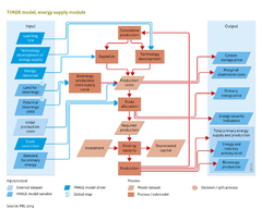
The structure of the biomass sub-model is similar to that of the fossil-fuel supply models, but with a few important differences ([[Hoogwijk, 2004]]) ([[***see Figure 4.1.3.1b]]). | The structure of the biomass sub-model is similar to that of the fossil-fuel supply models, but with a few important differences ([[Hoogwijk, 2004]]) ([[***see Figure 4.1.3.1b]]). | ||
* Depletion in the bio-energy model is not governed by cumulative production, but by the degree to which available land is being used for commercial energy crops. | * Depletion in the bio-energy model is not governed by cumulative production, but by the degree to which available land is being used for commercial energy crops. | ||
| Line 23: | Line 23: | ||
The production costs for bio-energy are represented by the costs of feedstock and conversion. Feedstock costs increase with actual production as a result of depletion; conversion costs, in contrast, decrease with cumulative production as a result of ‘learning by doing’. Feedstock costs include the costs of land, labour and capital. The costs of the conversion process include capital costs, O&M costs and the costs of energy use in this process. For both steps, the associated greenhouse gas emissions (related to deforestation, N2O from fertilisers, energy) are estimated ([[Emissions]]) and, where relevant, are subject to carbon tax. | The production costs for bio-energy are represented by the costs of feedstock and conversion. Feedstock costs increase with actual production as a result of depletion; conversion costs, in contrast, decrease with cumulative production as a result of ‘learning by doing’. Feedstock costs include the costs of land, labour and capital. The costs of the conversion process include capital costs, O&M costs and the costs of energy use in this process. For both steps, the associated greenhouse gas emissions (related to deforestation, N2O from fertilisers, energy) are estimated ([[Emissions]]) and, where relevant, are subject to carbon tax. | ||
===Other renewable energy=== | |||
The potential supply of renewable energy (wind, solar and bio-energy) is estimated in a generic way ([[Hoogwijk, 2004]]; [[De Vries et al., 2007]]): | The potential supply of renewable energy (wind, solar and bio-energy) is estimated in a generic way ([[Hoogwijk, 2004]]; [[De Vries et al., 2007]]): | ||
# First, the relevant physical and geographical data for the regions considered are collected on a 0.5 by 0.5 degree grid. The characteristics of wind speed, insulation and monthly variation are taken from the digital database constructed by the Climate Research Unit ([[New et al., 1997]]). Land use information for energy crops is taken from the [[Land cover and use|IMAGE land use model]]. | # First, the relevant physical and geographical data for the regions considered are collected on a 0.5 by 0.5 degree grid. The characteristics of wind speed, insulation and monthly variation are taken from the digital database constructed by the Climate Research Unit ([[New et al., 1997]]). Land use information for energy crops is taken from the [[Land cover and use|IMAGE land use model]]. | ||
Revision as of 13:50, 12 February 2014
Parts of Energy supply/Description
| Component is implemented in: |
|
| Related IMAGE components |
| Projects/Applications |
| Key publications |
| References |