Energy demand/Description: Difference between revisions
No edit summary |
Dafnomilii (talk | contribs) No edit summary |
||
| (57 intermediate revisions by 8 users not shown) | |||
| Line 1: | Line 1: | ||
{{ComponentDescriptionTemplate | {{ComponentDescriptionTemplate | ||
|Reference=De Vries et al., 2001; Richels et al., 2004; Van Ruijven et al., | |Reference=De Vries et al., 2001;Richels et al., 2004;Van Ruijven et al., 2016;Van Ruijven et al., 2011;Isaac and van Vuuren, 2009;Daioglou et al., 2014;Daioglou et al., 2022 | ||
}} | |||
<div class="page_standard"> | |||
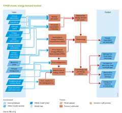
The energy demand module represents the total of all subsectors in the economy using energy, such as industry, transport, residential and services, etc. Each subsector is represented via either an aggregated formulation (used for the 'other' energy demand) or detailed modelling of specific processes (transport, residential and commercial and energy-intensive manufacturing industries - steel, cement, paper and pulp, food processing and non-energy). | |||
{{FormulaAndTableTemplate| | The generic formulation calculates total demand for final energy for each region (R), sector (S) and energy form (F, heat or electricity) according to: | ||
{{FormulaAndTableTemplate|Formula1 Energy demand}} | |||
Equation 1, in which: | |||
*SE represents final energy; | *SE represents final energy; | ||
*POP represents population; | *POP represents population; | ||
| Line 20: | Line 23: | ||
Population and economic activity levels are exogenous inputs into the module. Each of the other dynamic factors in equation 1 are briefly discussed below. | Population and economic activity levels are exogenous inputs into the module. Each of the other dynamic factors in equation 1 are briefly discussed below. | ||
===Structural change (SC)=== | ===Structural change (SC)=== | ||
In each sector, the mix of activities changes as a function of development and time. These changes, referred to as structural change, may influence the energy intensity of a sector. For instance, using more private cars for transport instead of buses tends to increase energy intensity. Historically, in several sectors, as a consequence of the structural changes in the type of activities an increase in energy intensity can be observed followed by a decrease. Evidence of this trend is more convincing in industry with shifts from very basic to heavy industry and finally to industries with high value-added products than in other sectors, such as transport where historically, energy intensity has mainly been increasing ([[De Vries et al., 2001]]). | In each sector, the mix of activities changes as a function of development and time. These changes, referred to as structural change, may influence the energy intensity of a sector. For instance, using more private cars for transport instead of buses tends to increase energy intensity. Historically, in several sectors, as a consequence of the structural changes in the type of activities an increase in energy intensity can be observed followed by a decrease. Evidence of this trend is more convincing in industry with shifts from very basic to heavy industry and finally to industries with high value-added products than in other sectors, such as transport where historically, energy intensity has mainly been increasing ([[De Vries et al., 2001]]). | ||
| Line 36: | Line 40: | ||
Demand for secondary energy carriers is determined on the basis of demand for energy services and the relative prices of the energy carriers. For each energy carrier, a final efficiency value (η) is assumed to account for differences between energy carriers in converting final energy into energy services. The indicated market share ([[HasAcronym::IMS]]) of each fuel is determined using a multinomial logit model that assigns market shares to the different carriers (i) on the basis of their relative prices in a set of competing carriers (j). | Demand for secondary energy carriers is determined on the basis of demand for energy services and the relative prices of the energy carriers. For each energy carrier, a final efficiency value (η) is assumed to account for differences between energy carriers in converting final energy into energy services. The indicated market share ([[HasAcronym::IMS]]) of each fuel is determined using a multinomial logit model that assigns market shares to the different carriers (i) on the basis of their relative prices in a set of competing carriers (j). | ||
{{FormulaAndTableTemplate| | {{FormulaAndTableTemplate|Formula2 Energy demand}} | ||
IMS is the indicated market share of different energy carriers or technologies and c is their costs. In this equation, λ is the so-called logit parameter, determining the sensitivity of markets to price differences. | IMS is the indicated market share of different energy carriers or technologies and c is their costs. In this equation, λ is the so-called logit parameter, determining the sensitivity of markets to price differences. | ||
The equation takes account of direct production costs and also energy and carbon taxes and premium values. The last two reflect non-price factors determining market shares, such as preferences, environmental policies, infrastructure (or the lack of infrastructure) and strategic considerations. The premium values are determined in the model calibration process in order to correctly simulate historical market shares on the basis of simulated price information. The same parameters are used in scenarios to simulate the assumption on societal preferences for clean and/or convenient fuels. However, the market shares of traditional biomass and secondary heat are determined by exogenous scenario parameters (except for the residential sector discussed below). Non-energy use of energy carriers is modelled on the basis of exogenously assumed intensity of representative non-energy uses (chemicals) and on a price-driven competition between the various energy carriers ([[Daioglou et al., | The equation takes account of direct production costs and also energy and carbon taxes and premium values. The last two reflect non-price factors determining market shares, such as preferences, environmental policies, infrastructure (or the lack of infrastructure) and strategic considerations. The premium values are determined in the model calibration process in order to correctly simulate historical market shares on the basis of simulated price information. The same parameters are used in scenarios to simulate the assumption on societal preferences for clean and/or convenient fuels. However, the market shares of traditional biomass and secondary heat are determined by exogenous scenario parameters (except for the residential sector discussed below). Non-energy use of energy carriers is modelled on the basis of exogenously assumed intensity of representative non-energy uses (chemicals) and on a price-driven competition between the various energy carriers ([[Daioglou et al., 2014]]). | ||
== | ===Industry=== | ||
The | The industry submodule includes representations for the steel, cement, non-energy (chemicals), pulp & paper and food processing sectors ([[Van Ruijven et al., 2016|Van Ruijven et al., 2016;]] [[Van Sluisveld et al., 2021]]). The generic structure of the energy demand module was adapted as follows: | ||
==Transport== | *Activity is described in terms of production of tonnes of product. The regional demand for these commodities is determined by a relationship similar to the formulation of the structural change discussed above. Cement and steel can be traded. Historically, trade patterns have been prescribed but future production is assumed to shift slowly to producers with the lowest costs. | ||
*The demand after trade can be met from production that uses a mix of production processes. Each production process is characterised by costs and energy use per unit of production, both of which decline slowly over time. The actual mix of production process used to produce feedstock or end product in the model is derived from a multinominal logit equation, and results in a larger market share for the production processes with the lowest costs. The autonomous improvement of these production processes leads to an autonomous increase in energy efficiency. The selection of production processes represents the price-induced improvement in energy efficiency. Fuel substitution is partly determined on the basis of price, but also depends on the type of production process used because some production processes can only use specific energy carriers (e.g., electricity for electric arc furnaces). | |||
More detailed information for specific manufacturing industries can be found in the Expert level of model documentation: http://image.int.pbl.nl/index.php/Expert:Energy_demand_-_Industry | |||
===== ''Non-Energy'' ===== | |||
The demand of energy carriers for non-energy purposes (feedstocks, chemicals) is modelled by determining the demand of four major end-use categories: Ammonia, Methanol, Higher Value Chemicals (benzene, toluene, xylene, etc.), and heavy refinery products. The future production of each of these categories is based on a relationship between historic production capacity and GDP growth, which is projected into the future. Specifically for Ammonia, a large portion of the demand is related to fertilizer use, endogenously driven by [[Agricultural economy/Description#Intensification of crop and pasture production|agricultural intensification]]. Different feedstocks (oil, gas, coal, bioenergy, recycled waste) compete to produce the annual non-energy demand based on their relative costs. Further details can be found at [[Daioglou et al., 2014|Daioglou et al., (2014)]] or in the Expert level of model documentation: http://image.int.pbl.nl/index.php/Expert:Energy_demand_-_Non-Energy | |||
===Transport=== | |||
The transport submodule consists of two parts - passenger and freight transport. A detailed description of the passenger transport (TRAVEL) is provided by Girod et al. ([[Girod et al., 2012|2012]]). There are seven modes - foot, bicycle, bus, train, passenger vehicle, high-speed train, and aircraft. The structural change (SC) processes in the transport module are described by an explicit consideration of the modal split. Two main factors govern model behaviour, namely the near-constancy of the travel time budget (TTB), and the travel money budget (TMB) over a large range of incomes. These are used as constraints to describe transition processes among the seven main travel modes, on the basis of their relative costs and speed characteristics and the consumer preferences for comfort levels and specific transport modes. | The transport submodule consists of two parts - passenger and freight transport. A detailed description of the passenger transport (TRAVEL) is provided by Girod et al. ([[Girod et al., 2012|2012]]). There are seven modes - foot, bicycle, bus, train, passenger vehicle, high-speed train, and aircraft. The structural change (SC) processes in the transport module are described by an explicit consideration of the modal split. Two main factors govern model behaviour, namely the near-constancy of the travel time budget (TTB), and the travel money budget (TMB) over a large range of incomes. These are used as constraints to describe transition processes among the seven main travel modes, on the basis of their relative costs and speed characteristics and the consumer preferences for comfort levels and specific transport modes. | ||
The freight transport submodule | The freight transport submodule contains a simpler structure. Service demand is projected with constant elasticity of the industry value added for each transport mode. In addition, demand sensitivity to transport prices is considered for each mode, depending on its share of energy costs in the total service costs. | ||
The efficiency changes in both passenger and freight transport represent the autonomous increase in energy efficiency, and the price-induced improvements in energy efficiency improvement parameters. These changes are described by substitution processes in explicit technologies, such as vehicles with different energy efficiencies, costs and fuel type characteristics compete on the basis of preferences and total passenger- | The efficiency changes in both passenger and freight transport represent the autonomous increase in energy efficiency, and the price-induced improvements in energy efficiency improvement parameters. These changes are described by substitution processes in explicit technologies, such as vehicles with different energy efficiencies, costs and fuel type characteristics compete on the basis of preferences and total passenger-kilometer costs, using a multinomial logit equation. The efficiency of the transport fleet is determined by a weighted average of the full fleet (a vintage model, giving an explicit description of the efficiency in all single years). As each type of vehicle is assumed to use only one fuel type, or in case of hybrid vehicles a fixed ratio of fuel types, this process also describes the fuel selection. | ||
Since Girod et. al ([[Girod et al., 2012|2012]]) the light duty vehicles (LDV) projected vehicle costs and efficiency have been revised to incorporate more recent projections of LDV vehicle technology development. The vehicle characteristics are based on the in depth study performed by the Argonne National Laboratory ([[Plotkin and Singh 2009|2009]]). Electric vehicle battery costs are updated based on Nykvist et al. ([[Nykvist2015|2015]]), which is described in Edelenbosch et al. ([[Edelenbosch et al. 2018|2018]]). | |||
=== Residential === | |||
The residential submodule describes the energy demand of households for a number of energy functions: ''cooking, appliances, space heating and cooling, water heating'', and ''lighting''. The model distinguishes five income quintiles for both the urban and rural populations. A representation of access to electricity and the associated investments is also included ([[Van Ruijven et al., 2012]]; [[Dagnachew et al., 2018]]). Projections for access to electricity are based on an econometric analysis that found a relationship between level of access, GDP per capita, and population density. The investment model is based on population density on a 0.5 x 0.5 degree grid, from which a stylised power grid is derived and analysed to determine investments in low-, medium- and high-voltage lines and transformers. See additional info on [[Grid and infrastructure|Grid and infrastructure.]] | |||
Structural change in energy demand is presented by modelling residential building stocks and their energy performance characteristics, as well as the demand for specific household energy functions. | |||
===== ''Building Stocks'' ===== | |||
Residential floorspace is modelled as a function of household expenditures with household size and per-capita floorspace. Together with overall population changes, this allows for projections of annual changes in floorspace. By attaching these annual changes with assumed building lifetimes, a stock model of residential buildings is constructed. | |||
The | Building stocks can have six possible insulation levels, with market shares of insulation levels determined via a [[Energy demand/Description#Substitution|multinomial logit function]]. The costs of each insulation level consist of the annualised capital costs, and the implied heating and cooling cost (savings). Thus, regions with higher heating/cooling requirements have increased incentive to invest in insulation. Existing building stocks can change their insulation level (i.e. renovate) 15 years after initial construction, with capital costs subject to discount rates associated with the remaining lifetime of the building ([[Daioglou et al., 2022]]). | ||
===== ''Energy Functions'' ===== | |||
*''<u>Space heating</u>'' energy demand is modelled using correlations with floor area, heating degree days and energy intensity, the last based on building insulation efficiency improvements (see [[Energy demand/Description#Building Stocks|Building Stocks]]). | |||
*''<u>Hot water</u>'' demand is modelled as a function of household income and heating degree days. | |||
*<u>''Cooking''</u> fuel use is determined on the basis of an requirement of 3 MJ<sub>UE</sub>/capita/day, kept constant across regions and time. | |||
*''<u>Appliances</u>'' energy demand is based on appliance ownership (disaggregated across 11 appliances), household income, efficiency reference values, and autonomous and price-induced improvements. | |||
*''<u>Space cooling</u>'' has a similar approach to appliances but also accounts for cooling degree days which determine the maximum cooling demand (Isaac and Van Vuuren, 2009). | |||
*''<u>Lighting</u>'' electricity use is determined on the basis of floor area, wattage and lighting hours based on geographic location. | |||
These functions are described in detail elsewhere ([[Daioglou et al., 2012]]; [[Van Ruijven et al., 2011]]). After determining the energy demand per function for each population quintile, the choice of fuel type is determined on the basis of relative costs. This is based on a [[Energy demand/Description#Substitution|multinomial logit formulation]] for energy functions that can involve multiple fuels, such as cooking and space heating. In the calculations, consumer discount rates are assumed to decrease along with household income levels, and there will be increasing appreciation of clean and convenient fuels ([[Van Ruijven et al., 2011]]). For developing countries, this endogenously results in the substitution processes described by the energy ladder. This refers to the progressive use of modern energy types as incomes grow, from traditional bioenergy to coal and kerosene, to energy carriers such as natural gas, heating oil and electricity. | |||
===== ''Efficiency Improvement'' ===== | |||
Efficiency improvements of useful and final energy demand are included in different ways. Exogenously driven energy efficiency improvement over time are used for appliances, light bulbs, air conditioning, and heating equipment. Price-induced energy efficiency improvements (PIEEI) - in all energy functions - can occur due to changing competitiveness of different options as relative energy prices change. For example, changes in the price of electricity affects the competition between incandescent light bulbs and more energy-efficient (but capital intensive) lighting. For appliances, there is a stylized relationship between increased electricity prices and ''Unit Energy Consumption'' ''(kWh/yr).'' Changes in energy prices and associated heating and cooling costs also affect renovation rates and incentives to improve building-shell efficiency ([[Daioglou et al., 2022]]). Stocks of all energy consuming equipment are tracked by attaching a technical lifetime to them, after which they may be replaced. | |||
Projected building stocks and electricity prices also affect the possibility to invest in rooftop PV, thus allowing residential building to also acts as "prosumers" of electricity (see: [[Energy supply/Description]]). | |||
=== Services & Commercial === | |||
Energy demand of the services & commercial sector is related to changes in value added of the service sector (related to GDP changes). Energy demand of this sector is disaggregated across six energy functions: ''Space heating, space cooling, water heating, cooking, lighting, appliances & general electricity.'' For the heating and cooking functions, there are representative technologies for different fuels (coal, oil, gas, modern biofuel, hydrogen, district heat, electricity) compete based on their relative costs. For ''space cooling, lighting,'' and ''appliances'' only electricity can be used. | |||
</div> | |||
<references /> | |||
Latest revision as of 11:51, 18 November 2022
Parts of Energy demand/Description
| Component is implemented in: |
|
| Related IMAGE components |
| Projects/Applications |
| Key publications |
| References |
Model description of Energy demand
The energy demand module represents the total of all subsectors in the economy using energy, such as industry, transport, residential and services, etc. Each subsector is represented via either an aggregated formulation (used for the 'other' energy demand) or detailed modelling of specific processes (transport, residential and commercial and energy-intensive manufacturing industries - steel, cement, paper and pulp, food processing and non-energy).
The generic formulation calculates total demand for final energy for each region (R), sector (S) and energy form (F, heat or electricity) according to:
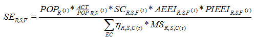
Equation 1, in which:
- SE represents final energy;
- POP represents population;
- ACT/POP the sectoral activity per capita;
- SC a factor capturing intra-sectoral structural change;
- AEEI the autonomous energy efficiency improvement;
- PIEEI the price-induced energy efficiency improvement.
In the denominator:
- η is the end-use efficiency of energy carriers used in, for example, boilers and stoves;
- MS represents the share of each energy carrier.
Population and economic activity levels are exogenous inputs into the module. Each of the other dynamic factors in equation 1 are briefly discussed below.
Structural change (SC)
In each sector, the mix of activities changes as a function of development and time. These changes, referred to as structural change, may influence the energy intensity of a sector. For instance, using more private cars for transport instead of buses tends to increase energy intensity. Historically, in several sectors, as a consequence of the structural changes in the type of activities an increase in energy intensity can be observed followed by a decrease. Evidence of this trend is more convincing in industry with shifts from very basic to heavy industry and finally to industries with high value-added products than in other sectors, such as transport where historically, energy intensity has mainly been increasing (De Vries et al., 2001).
Based on the above, in generic model formulations, energy intensity is driven by income, assuming a peak in energy intensity, followed by saturation of energy demand at a constant per capita energy service level. In the calibration process, the choice of parameters may lead, for instance, to a peak in energy intensity higher than current income levels. In the technology-detailed energy demand (see below), structural change is captured by other equations that describe the underlying processes explicitly (e.g., modal shift in transport).
Autonomous Energy Efficiency Increase (AEEI)
This is a multiplier used in the generic energy demand module to account for efficiency improvement as a result of technology improvement, independent of prices. In general, current appliances are more efficient than those available in the past.
The autonomous energy efficiency increase for new capital is a fraction (f) of the economic growth rate based on the formulation of Richels et al. (2004). The fraction varies between 0.45 and 0.30 (based on literature data) and is assumed to decline with time because the scope for further improvement is assumed to decline. Efficiency improvement is assumed for new capital. Autonomous increase in energy efficiency for the average capital stock is calculated as the weighted average value of the AEEI values of the total in capital stock, using the vintage formulation. In the technology-detailed submodules, the autonomous energy efficiency increase is represented by improvement in individual technologies over time.
Price-Induced Energy Efficiency Improvement (PIEEI)
This multiplier is used to describe the effect of rising energy costs in the form of induced investments in energy efficiency by consumers. It is included in the generic formulation using an energy conservation cost curve. In the technology-detailed submodules, this multiplier is represented by competing technologies with different efficiencies and costs.
Substitution
Demand for secondary energy carriers is determined on the basis of demand for energy services and the relative prices of the energy carriers. For each energy carrier, a final efficiency value (η) is assumed to account for differences between energy carriers in converting final energy into energy services. The indicated market share (IMS) of each fuel is determined using a multinomial logit model that assigns market shares to the different carriers (i) on the basis of their relative prices in a set of competing carriers (j).
IMS is the indicated market share of different energy carriers or technologies and c is their costs. In this equation, λ is the so-called logit parameter, determining the sensitivity of markets to price differences.
The equation takes account of direct production costs and also energy and carbon taxes and premium values. The last two reflect non-price factors determining market shares, such as preferences, environmental policies, infrastructure (or the lack of infrastructure) and strategic considerations. The premium values are determined in the model calibration process in order to correctly simulate historical market shares on the basis of simulated price information. The same parameters are used in scenarios to simulate the assumption on societal preferences for clean and/or convenient fuels. However, the market shares of traditional biomass and secondary heat are determined by exogenous scenario parameters (except for the residential sector discussed below). Non-energy use of energy carriers is modelled on the basis of exogenously assumed intensity of representative non-energy uses (chemicals) and on a price-driven competition between the various energy carriers (Daioglou et al., 2014).
Industry
The industry submodule includes representations for the steel, cement, non-energy (chemicals), pulp & paper and food processing sectors (Van Ruijven et al., 2016; Van Sluisveld et al., 2021). The generic structure of the energy demand module was adapted as follows:
- Activity is described in terms of production of tonnes of product. The regional demand for these commodities is determined by a relationship similar to the formulation of the structural change discussed above. Cement and steel can be traded. Historically, trade patterns have been prescribed but future production is assumed to shift slowly to producers with the lowest costs.
- The demand after trade can be met from production that uses a mix of production processes. Each production process is characterised by costs and energy use per unit of production, both of which decline slowly over time. The actual mix of production process used to produce feedstock or end product in the model is derived from a multinominal logit equation, and results in a larger market share for the production processes with the lowest costs. The autonomous improvement of these production processes leads to an autonomous increase in energy efficiency. The selection of production processes represents the price-induced improvement in energy efficiency. Fuel substitution is partly determined on the basis of price, but also depends on the type of production process used because some production processes can only use specific energy carriers (e.g., electricity for electric arc furnaces).
More detailed information for specific manufacturing industries can be found in the Expert level of model documentation: http://image.int.pbl.nl/index.php/Expert:Energy_demand_-_Industry
Non-Energy
The demand of energy carriers for non-energy purposes (feedstocks, chemicals) is modelled by determining the demand of four major end-use categories: Ammonia, Methanol, Higher Value Chemicals (benzene, toluene, xylene, etc.), and heavy refinery products. The future production of each of these categories is based on a relationship between historic production capacity and GDP growth, which is projected into the future. Specifically for Ammonia, a large portion of the demand is related to fertilizer use, endogenously driven by agricultural intensification. Different feedstocks (oil, gas, coal, bioenergy, recycled waste) compete to produce the annual non-energy demand based on their relative costs. Further details can be found at Daioglou et al., (2014) or in the Expert level of model documentation: http://image.int.pbl.nl/index.php/Expert:Energy_demand_-_Non-Energy
Transport
The transport submodule consists of two parts - passenger and freight transport. A detailed description of the passenger transport (TRAVEL) is provided by Girod et al. (2012). There are seven modes - foot, bicycle, bus, train, passenger vehicle, high-speed train, and aircraft. The structural change (SC) processes in the transport module are described by an explicit consideration of the modal split. Two main factors govern model behaviour, namely the near-constancy of the travel time budget (TTB), and the travel money budget (TMB) over a large range of incomes. These are used as constraints to describe transition processes among the seven main travel modes, on the basis of their relative costs and speed characteristics and the consumer preferences for comfort levels and specific transport modes.
The freight transport submodule contains a simpler structure. Service demand is projected with constant elasticity of the industry value added for each transport mode. In addition, demand sensitivity to transport prices is considered for each mode, depending on its share of energy costs in the total service costs.
The efficiency changes in both passenger and freight transport represent the autonomous increase in energy efficiency, and the price-induced improvements in energy efficiency improvement parameters. These changes are described by substitution processes in explicit technologies, such as vehicles with different energy efficiencies, costs and fuel type characteristics compete on the basis of preferences and total passenger-kilometer costs, using a multinomial logit equation. The efficiency of the transport fleet is determined by a weighted average of the full fleet (a vintage model, giving an explicit description of the efficiency in all single years). As each type of vehicle is assumed to use only one fuel type, or in case of hybrid vehicles a fixed ratio of fuel types, this process also describes the fuel selection.
Since Girod et. al (2012) the light duty vehicles (LDV) projected vehicle costs and efficiency have been revised to incorporate more recent projections of LDV vehicle technology development. The vehicle characteristics are based on the in depth study performed by the Argonne National Laboratory (2009). Electric vehicle battery costs are updated based on Nykvist et al. (2015), which is described in Edelenbosch et al. (2018).
Residential
The residential submodule describes the energy demand of households for a number of energy functions: cooking, appliances, space heating and cooling, water heating, and lighting. The model distinguishes five income quintiles for both the urban and rural populations. A representation of access to electricity and the associated investments is also included (Van Ruijven et al., 2012; Dagnachew et al., 2018). Projections for access to electricity are based on an econometric analysis that found a relationship between level of access, GDP per capita, and population density. The investment model is based on population density on a 0.5 x 0.5 degree grid, from which a stylised power grid is derived and analysed to determine investments in low-, medium- and high-voltage lines and transformers. See additional info on Grid and infrastructure.
Structural change in energy demand is presented by modelling residential building stocks and their energy performance characteristics, as well as the demand for specific household energy functions.
Building Stocks
Residential floorspace is modelled as a function of household expenditures with household size and per-capita floorspace. Together with overall population changes, this allows for projections of annual changes in floorspace. By attaching these annual changes with assumed building lifetimes, a stock model of residential buildings is constructed.
Building stocks can have six possible insulation levels, with market shares of insulation levels determined via a multinomial logit function. The costs of each insulation level consist of the annualised capital costs, and the implied heating and cooling cost (savings). Thus, regions with higher heating/cooling requirements have increased incentive to invest in insulation. Existing building stocks can change their insulation level (i.e. renovate) 15 years after initial construction, with capital costs subject to discount rates associated with the remaining lifetime of the building (Daioglou et al., 2022).
Energy Functions
- Space heating energy demand is modelled using correlations with floor area, heating degree days and energy intensity, the last based on building insulation efficiency improvements (see Building Stocks).
- Hot water demand is modelled as a function of household income and heating degree days.
- Cooking fuel use is determined on the basis of an requirement of 3 MJUE/capita/day, kept constant across regions and time.
- Appliances energy demand is based on appliance ownership (disaggregated across 11 appliances), household income, efficiency reference values, and autonomous and price-induced improvements.
- Space cooling has a similar approach to appliances but also accounts for cooling degree days which determine the maximum cooling demand (Isaac and Van Vuuren, 2009).
- Lighting electricity use is determined on the basis of floor area, wattage and lighting hours based on geographic location.
These functions are described in detail elsewhere (Daioglou et al., 2012; Van Ruijven et al., 2011). After determining the energy demand per function for each population quintile, the choice of fuel type is determined on the basis of relative costs. This is based on a multinomial logit formulation for energy functions that can involve multiple fuels, such as cooking and space heating. In the calculations, consumer discount rates are assumed to decrease along with household income levels, and there will be increasing appreciation of clean and convenient fuels (Van Ruijven et al., 2011). For developing countries, this endogenously results in the substitution processes described by the energy ladder. This refers to the progressive use of modern energy types as incomes grow, from traditional bioenergy to coal and kerosene, to energy carriers such as natural gas, heating oil and electricity.
Efficiency Improvement
Efficiency improvements of useful and final energy demand are included in different ways. Exogenously driven energy efficiency improvement over time are used for appliances, light bulbs, air conditioning, and heating equipment. Price-induced energy efficiency improvements (PIEEI) - in all energy functions - can occur due to changing competitiveness of different options as relative energy prices change. For example, changes in the price of electricity affects the competition between incandescent light bulbs and more energy-efficient (but capital intensive) lighting. For appliances, there is a stylized relationship between increased electricity prices and Unit Energy Consumption (kWh/yr). Changes in energy prices and associated heating and cooling costs also affect renovation rates and incentives to improve building-shell efficiency (Daioglou et al., 2022). Stocks of all energy consuming equipment are tracked by attaching a technical lifetime to them, after which they may be replaced.
Projected building stocks and electricity prices also affect the possibility to invest in rooftop PV, thus allowing residential building to also acts as "prosumers" of electricity (see: Energy supply/Description).
Services & Commercial
Energy demand of the services & commercial sector is related to changes in value added of the service sector (related to GDP changes). Energy demand of this sector is disaggregated across six energy functions: Space heating, space cooling, water heating, cooking, lighting, appliances & general electricity. For the heating and cooking functions, there are representative technologies for different fuels (coal, oil, gas, modern biofuel, hydrogen, district heat, electricity) compete based on their relative costs. For space cooling, lighting, and appliances only electricity can be used.