Energy supply/Description

Component is implemented in:

TIMER model (version TIMER 3.2) Aggregated component: Energy supply and demand Components: Emissions Energy conversion Energy demand Energy supply

Related IMAGE components

Atmospheric composition and climate Climate policy Crops and grass Drivers Land cover and land use

Projects/Applications

ADVANCE project Roads from Rio+20 (2012) project

Key publications

De Vries et al., 2007 Van Vuuren et al., 2008 Van Vuuren et al., 2009

References

Daioglou et al., 2019 De Vries et al., 2007 Gernaat et al., 2014 Gernaat et al., 2017 Gernaat et al., 2021 Hoogwijk, 2004 Köberle et al., 2015

Flowchart Energy supply. See also the Input/Output Table on the introduction page.

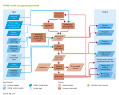
Model description of Energy supply

Model description of Energy supply

Fossil fuels and uranium

Depletion of fossil fuels (coal, oil and natural gas) and uranium is simulated on the assumption that resources can be represented by a long-term supply cost curve, consisting of different resource categories with increasing costs levels. The model assumes that the cheapest deposits will be exploited first. For each region, there are 12 resource categories for oil, gas and nuclear fuels, and 14 categories for coal.

A key input for each of the fossil fuel and uranium supply submodules is fuel demand (fuel used in final energy and conversion processes). Additional input includes conversion losses in refining, liquefaction, conversion, and energy use in the energy system. [!CHANGE] Upstream energy use is endogenously determined based energy carrier, region in which the energy carrier is produced, production rate and resource category. These submodules indicate how demand can be met by supply in a region and other regions through interregional trade.

Table: [!CHANGE]Main assumptions on fossil fuel resources (in ZJ; coal does not have a distinction between conventional and unconventional; Rogner, 1997; Mulders et al., 2006; [[IEA, 2017]], [[USGS, 2012]]; [[BGR, 2016]]; EDGAR database; [[Abundant Gas Project]])

	Oil	Natural gas	Underground coal	Surface coal
Cum. 1970-2015 production	6.5	3.4	2.4	1.5
Reserves	9.4	7.3	17	3.6
Other conventional resources	33	17	481	56
Unconventional resources (reserves)	2.0	0.30
Other unconventional resources	54	2023
Total	105	2051	501	61

Fossil fuel resources are aggregated to five resource categories for each fuel (the table above). Each category has typical production costs. The resource estimates for oil and natural gas supply imply that for conventional resources supply is limited to only [!CHANGE] about 7 times the 1970–2015 production level. Production estimates for unconventional resources are much larger, albeit very speculative. Recently, some of the occurrences of these unconventional resources have become competitive such as shale gas and tar sands. For coal, even current reserves amount to almost ten times the production level of the last three decades. For all fuels, the model assumes that, if prices increase, or if there is further technology development, the energy could be produced in the higher cost resource categories. The values presented in the table above represent medium estimates in the model, which can also use higher or lower estimates in the scenarios. The final production costs in each region are determined by the combined effect of resource depletion and learning-by-doing.

Trade

Trade is dealt with in a generic way for oil, natural gas and coal. In the fuel trade model, each region imports fuels from other regions. The amount of fuel imported from each region depends on the relative production costs and those in other regions, augmented with transport costs, using multinomial logit equations. Transport costs are calculated from representative interregional transport distances and time- and fuel-dependent estimates of the costs per GJ per kilometre.

To reflect geographical, political and other constraints in the interregional fuel trade, an additional 'cost' is added to simulate trade barriers between regions (this costs factor is determined by calibration). Natural gas is transported by pipeline or liquid-natural gas (LNG) tanker, depending on distance, with pipeline more attractive for short distances. In order to account for cartel behaviour, the model compares production costs with and without unrestricted trade. Regions that can supply at lower costs than the average production costs in importing regions are assumed to supply oil at a price only slightly below the production costs of the importing regions. Although also this rule is implemented in a generic form for all energy carriers, it is only effective for oil, where the behaviour of the OPEC cartel is simulated to some extent.

Bioenergy

The structure of the biomass submodule is similar to that for fossil fuel supply, but with the following differences (Hoogwijk, 2004):

• Depletion of bioenergy is not governed by cumulative production but by the degree to which available land is used for commercial energy crops.
• The total amount of potentially available bioenergy is derived from bioenergy crop yields calculated on a 0.5x0.5 degree grid with the IMAGE crop model for various land-use scenarios for the 21st century. Potential supply is restricted on the basis of a set of criteria, the most important of which is that bioenergy crops can only be on abandoned agricultural land and on part of the natural grassland. The costs of primary bioenergy crops (woody, grassy, maize and sugar cane) are calculated with a Cobb-Douglas economic growth model using labour , land rent and capital costs as inputs. The land costs are based on average regional income levels per km², which was found to be a reasonable proxy for regional differences in land rent costs. The production functions are calibrated to empirical data (Hoogwijk, 2004).
• The model describes the conversion of biomass (including residues, in addition to wood crops, grassy crops, maize and sugar cane) to two generic secondary fuel types: bio-solid fuels used in the industry and power sectors; and liquid fuel used mostly in the transport sector.
• The trade and allocation of biofuel production to regions is determined by optimisation. An optimal mix of bio-solid and bio-liquid fuel supply across regions is calculated, using the prices of the previous time step to calculate the demand.

The production costs for bioenergy are represented by the costs of feedstock and conversion. Feedstock costs increase with actual production as a result of depletion, while conversion costs decrease with cumulative production as a result of ‘learning by doing’. Feedstock costs include the costs of land, labour and capital, while conversion costs include capital, O&M and energy use in this process. For both steps, the associated greenhouse gas emissions (related to spatially explicit land use change, N₂O from fertilisers, energy) are estimated (see Component Emissions), and are subject to carbon tax, where relevant .

Besides the energy crops mentioned above, agricultural and forestry residues can also be used as a primary feedstock for modern bioenergy. The availability of residues is linked to the productivity of agriculture and forestry, taking into account the effect of changing yields (see Agricultural economy description) or Forest management techniques. The available potential is limited by environmental constraints as well as competing uses (use of agricultural residues as feed for livestock, see Agricultural economy). As with bioenergy crops, availability and costs of residues are calculated on a 0.5x0.5 degree grid.

Other renewable energy

Potential supply of renewable energy (wind, solar and bioenergy) is estimated generically as follows (Hoogwijk, 2004; De Vries et al., 2007):

1. Physical and geographical data for the regions considered are collected on a 0.5x0.5 degree grid. The characteristics of wind speed, insulation and monthly variation are taken from the digital database constructed by the Climate Research Unit (New et al., 1997).
2. The model assesses the part of the grid cell that can be used for energy production, given its physical–geographic (terrain, habitation) and socio-geographical (location, acceptability) characteristics. This leads to an estimate of the geographical potential. Several of these factors are scenario-dependent. The geographical potential for biomass production from energy crops is estimated using suitability/availability factors taking account of competing land-use options and the harvested rain-fed yield of energy crops.
3. Next, we assume that only part of the geographical potential can be used due to limited conversion efficiency and maximum power density, This result of accounting for these conversion efficiencies is referred to as the technical potential.
4. The final step is to relate the technical potential to on-site production costs. Information at grid level is sorted and used as supply cost curves to reflect the assumption that the lowest cost locations are exploited first. Supply cost curves are used dynamically and change over time as a result of the learning effect.