Emissions/Description: Difference between revisions
Jump to navigation
Jump to search
No edit summary |
No edit summary |
||
| Line 1: | Line 1: | ||
{{ComponentDescriptionTemplate | {{ComponentDescriptionTemplate | ||
|Reference=IPCC, 2006; Cofala et al., 2002; Stern, 2003; Smith et al., 2005; Van Ruijven et al., 2008; Carson, 2010; Smith et al., 2011; Bouwman et al., 2002; Bouwman et al., 1993; Harnisch et al.,2009a; Harnisch et al., 2009b; Velders et al., 2009; Bouwman, 1994; Bouwman et al., 1997; Bouwman et al., 2002a; Braspenning Radu et al., 2012; | |Reference=IPCC, 2006; Cofala et al., 2002; Stern, 2003; Smith et al., 2005; Van Ruijven et al., 2008; Carson, 2010; Smith et al., 2011; Bouwman et al., 2002; Bouwman et al., 1993; Harnisch et al.,2009a; Harnisch et al., 2009b; Velders et al., 2009; Kreileman and Bouwman, 1994; Bouwman et al., 1997; Bouwman et al., 2002a; Braspenning Radu et al., 2012; | ||
|Description===General approaches== | |Description===General approaches== | ||
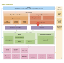
[[Table 5.1]] lists the different sources of emissions included in the IMAGE model. Emissions that are transported in water (nitrate, phosphorus) are discussed in [[Nutrient balances]]. Regarding the approach and spatial detail for modeling gaseous emissions, IMAGE uses four different ways to represent emissions. | [[Table 5.1]] lists the different sources of emissions included in the IMAGE model. Emissions that are transported in water (nitrate, phosphorus) are discussed in [[Nutrient balances]]. Regarding the approach and spatial detail for modeling gaseous emissions, IMAGE uses four different ways to represent emissions. | ||
| Line 7: | Line 7: | ||
The equation for this emission factor approach is as follows: | The equation for this emission factor approach is as follows: | ||
Emission = Activityr,I * EF-baser,i * AF r,i ([[5.1]]) | [[Emission = Activityr,I * EF-baser,i * AF r,i ([[5.1]]) ]] | ||
where Emission is the emission of the specific gas; Activity is the Energy input or agricultural activity, r is the index for region, i index for further specification (sector, energy carrier), EF-base is the emission factor in the baseline and AF is the abatement factor, i.e. the reduction of the baseline emission factor as a result of climate policy. The emission factors are time-dependent, representing changes in technology and air pollution control policies. | where Emission is the emission of the specific gas; Activity is the Energy input or agricultural activity, r is the index for region, i index for further specification (sector, energy carrier), EF-base is the emission factor in the baseline and AF is the abatement factor, i.e. the reduction of the baseline emission factor as a result of climate policy. The emission factors are time-dependent, representing changes in technology and air pollution control policies. | ||
| Line 15: | Line 15: | ||
* ''Emission factor method with spatial distribution'' (GEF) represents a special case of the EF method where a proxy distribution is used to present gridded emissions. This is done for a number of sources, for example emissions from animals ([[Table 5.1]]). | * ''Emission factor method with spatial distribution'' (GEF) represents a special case of the EF method where a proxy distribution is used to present gridded emissions. This is done for a number of sources, for example emissions from animals ([[Table 5.1]]). | ||
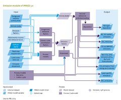
* ''Process model''. (GPM). Land-use related emissions of NH3, N2O and NO are calculated with grid-specific models. The models included in IMAGE are simple regression models that generate an emission factor ([[Figure 5.1]]). It should be noted that for comparison with other models, IMAGE also includes the N2O methodology as proposed by [[IPCC]] ([[IPCC, 2006]]). | |||
The approaches used for emissions from energy production and use, industrial processes and land-use related sources are discussed in more detail below. | The approaches used for emissions from energy production and use, industrial processes and land-use related sources are discussed in more detail below. | ||
| Line 22: | Line 22: | ||
Emission factors (EFs) ([[equation 5.1]]) are used to estimate emissions from the various energy-related sources ([[Table 5.2]]). In general, the so-called Tier 1 approach from IPCC guidelines ([[IPCC, 2006]]) is used. In the energy system, emissions are calculated by multiplying energy use fluxes with time-dependent emission factors. Changes in the emission factors represent technological improvements and end of-pipe control techniques, fuel specification standards for transport, clean-coal technologies in industry, etc. | Emission factors (EFs) ([[equation 5.1]]) are used to estimate emissions from the various energy-related sources ([[Table 5.2]]). In general, the so-called Tier 1 approach from IPCC guidelines ([[IPCC, 2006]]) is used. In the energy system, emissions are calculated by multiplying energy use fluxes with time-dependent emission factors. Changes in the emission factors represent technological improvements and end of-pipe control techniques, fuel specification standards for transport, clean-coal technologies in industry, etc. | ||
The emission factors are calibrated for the historical period on the basis of the EDGAR emission model as described by [[Braspenning Radu et al., 2012]]. The calibration to the EDGAR database is not always straightforward due to differences in aggregation level. The general rule is to use weighted average emission factors in the case of aggregation. However, in those cases in which this results in incomprehensible emission factors (in particular when large differences exists between the emission factors for the underlying technologies) specific emission factors were chosen. | The emission factors are calibrated for the historical period on the basis of the [[EDGAR model|EDGAR emission model]] as described by [[Braspenning Radu et al., 2012]]. The calibration to the EDGAR database is not always straightforward due to differences in aggregation level. The general rule is to use weighted average emission factors in the case of aggregation. However, in those cases in which this results in incomprehensible emission factors (in particular when large differences exists between the emission factors for the underlying technologies) specific emission factors were chosen. | ||
==Future emission factors are based on different rules:== | ==Future emission factors are based on different rules:== | ||
| Line 39: | Line 39: | ||
==Emissions from industrial processes== | ==Emissions from industrial processes== | ||
For the industrial sector, the energy model includes several activity levels that determine emissions. These can divided into three categories: | For the industrial sector, the energy model includes several activity levels that determine emissions. These can divided into three categories: | ||
* Cement and steel production. For these commodities, IMAGE-TIMER actually includes detailed demand models ([[Energy supply and demand]]). Similar to energy, the emissions are calculated by multiplying the activity levels to exogenously set emission factors. | |||
* Other industrial activities. Here the activity levels are formulated as a regional function of industrial value added. Activity levels include for instance copper production, and the production of solvents. Again, emissions are calculated by multiplying the activity levels with emission factors. | |||
* For the halogenated gases, finally we have implemented the approach developed by [[Harnisch et al.,2009a]]. They derived relationships with income for the main uses of halogenated gasses (HFCs, PFCs, SF6). In the actual use of the model, slightly updated parameters are used to better represent the projections as presented by [[Velders et al., 2009]]. The marginal abatement cost curve per gas still follows the methodology described by [[Harnisch et al., 2009b]]. | |||
==Land-use related emissions== | ==Land-use related emissions== | ||
| Line 50: | Line 50: | ||
Constant emission factors may lead to decreasing emissions per unit of product, for example when the emission factor is specified on a per head basis. An increasing production per head may then lead to a decreasing emission per unit of product. An example is the constant CH4 emission from animal waste per animal, which leads to decreasing emissions per unit of meat or milk when the production per animal increases. | Constant emission factors may lead to decreasing emissions per unit of product, for example when the emission factor is specified on a per head basis. An increasing production per head may then lead to a decreasing emission per unit of product. An example is the constant CH4 emission from animal waste per animal, which leads to decreasing emissions per unit of meat or milk when the production per animal increases. | ||
A special case is the N2O emission after forest clearing. Deforestation may lead to accelerated decomposition of litter, root material and loss of part of soil organic matter in the first year after the clearing, causing a pulse of N2O emissions. To mimic this effect, emissions in the first year after clearing are assumed to be 5 times the flux in the original ecosystem. They decrease linearly to the level of the new ecosystem in the 10th year, usually lower than the flux in the original forest. More details can be found in Kreileman and | A special case is the N2O emission after forest clearing. Deforestation may lead to accelerated decomposition of litter, root material and loss of part of soil organic matter in the first year after the clearing, causing a pulse of N2O emissions. To mimic this effect, emissions in the first year after clearing are assumed to be 5 times the flux in the original ecosystem. They decrease linearly to the level of the new ecosystem in the 10th year, usually lower than the flux in the original forest. More details can be found in [[Kreileman and Bouwman, 1994]]. | ||
Land-use related emissions of NH3, N2O and NO are calculated with a grid-specific model, N2O from soils under natural vegetation is calculated with the model of [[Bouwman et al., 1993]]. This model is a regression model based on temperature, a proxy for soil carbon input, soil water and oxygen status and a proxy for net primary production. Ammonia emission from natural vegetation is based on net primary production, C:Nratio and an emission factor, and the model accounts for in-canopy retention of the emitted NH3 ([[Bouwman et al., 1997]]). | Land-use related emissions of NH3, N2O and NO are calculated with a grid-specific model, N2O from soils under natural vegetation is calculated with the model of [[Bouwman et al., 1993]]. This model is a regression model based on temperature, a proxy for soil carbon input, soil water and oxygen status and a proxy for net primary production. Ammonia emission from natural vegetation is based on net primary production, C:Nratio and an emission factor, and the model accounts for in-canopy retention of the emitted NH3 ([[Bouwman et al., 1997]]). | ||
| Line 60: | Line 60: | ||
==Emission abatement== | ==Emission abatement== | ||
Future emissions for a number of energy and land-use related sources also vary in future years as a result of climate policy. This is described by using so-called abatement coefficients ([[Figure 5.1]]). The values of these coefficients depend on the scenario assumptions. In scenarios in which climate change or sustainability is an important feature in the storyline, abatement will be more important than in business-as-usual scenarios. Abatement factors are used in particular for CH4 emissions from fossil fuel production and transport, N2O emissions from transport and for CH4 emissions from enteric fermentation and from animal waste, and N2O emissions from animal waste according to the IPCC method. These abatement files are calculated in the climate policy submodel of IMAGE on the basis of comparing the costs of non-CO2 abatement in agriculture against other mitigation options. | Future emissions for a number of energy and land-use related sources also vary in future years as a result of climate policy. This is described by using so-called abatement coefficients ([[Figure 5.1]]). The values of these coefficients depend on the scenario assumptions. In scenarios in which climate change or sustainability is an important feature in the storyline, abatement will be more important than in business-as-usual scenarios. Abatement factors are used in particular for CH4 emissions from fossil fuel production and transport, N2O emissions from transport and for CH4 emissions from enteric fermentation and from animal waste, and N2O emissions from animal waste according to the IPCC method. These abatement files are calculated in the climate policy submodel of IMAGE on the basis of comparing the costs of non-CO2 abatement in agriculture against other mitigation options. | ||
}} | }} | ||
Revision as of 10:30, 15 January 2014
Parts of Emissions/Description
| Component is implemented in: |
Components:and
|
| Projects/Applications |
| Models/Databases |
| Key publications |
| References |
|