Emissions/Description: Difference between revisions
Jump to navigation
Jump to search
No edit summary |
No edit summary |
||
| Line 1: | Line 1: | ||
{{ComponentDescriptionTemplate | {{ComponentDescriptionTemplate | ||
|Reference=IPCC, 2006; Cofala et al., 2002; Stern, 2003; Smith et al., 2005; Van Ruijven et al., 2008; Carson, 2010; Smith et al., 2011; | |Reference=IPCC, 2006; Cofala et al., 2002; Stern, 2003; Smith et al., 2005; Van Ruijven et al., 2008; Carson, 2010; Smith et al., 2011; Bouwman et al., 1993; Harnisch et al., 2009; Velders et al., 2009; Kreileman and Bouwman, 1994; Bouwman et al., 1997; Bouwman et al., 2002a; Braspenning Radu et al., 2012; | ||
|Description===General approaches== | |Description===General approaches== | ||
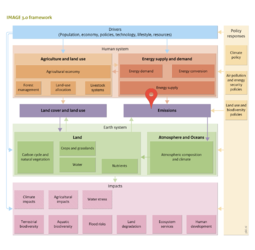
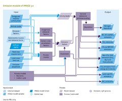
[[Table 5.1]] lists the different sources of emissions included in the IMAGE model. Emissions that are transported in water (nitrate, phosphorus) are discussed in [[Nutrient balances]]. Regarding the approach and spatial detail for modeling gaseous emissions, IMAGE uses four different ways to represent emissions. | [[Table 5.1]] lists the different sources of emissions included in the IMAGE model. Emissions that are transported in water (nitrate, phosphorus) are discussed in [[Nutrient balances]]. Regarding the approach and spatial detail for modeling gaseous emissions, IMAGE uses four different ways to represent emissions. | ||
| Line 41: | Line 41: | ||
* Cement and steel production. For these commodities, IMAGE-TIMER actually includes detailed demand models ([[Energy supply and demand]]). Similar to energy, the emissions are calculated by multiplying the activity levels to exogenously set emission factors. | * Cement and steel production. For these commodities, IMAGE-TIMER actually includes detailed demand models ([[Energy supply and demand]]). Similar to energy, the emissions are calculated by multiplying the activity levels to exogenously set emission factors. | ||
* Other industrial activities. Here the activity levels are formulated as a regional function of industrial value added. Activity levels include for instance copper production, and the production of solvents. Again, emissions are calculated by multiplying the activity levels with emission factors. | * Other industrial activities. Here the activity levels are formulated as a regional function of industrial value added. Activity levels include for instance copper production, and the production of solvents. Again, emissions are calculated by multiplying the activity levels with emission factors. | ||
* For the halogenated gases, finally we have implemented the approach developed by [[Harnisch et al., | * For the halogenated gases, finally we have implemented the approach developed by [[Harnisch et al.,2009]]. They derived relationships with income for the main uses of halogenated gasses (HFCs, PFCs, SF6). In the actual use of the model, slightly updated parameters are used to better represent the projections as presented by [[Velders et al., 2009]]. The marginal abatement cost curve per gas still follows the methodology described by [[Harnisch et al., 2009]]. | ||
==Land-use related emissions== | ==Land-use related emissions== | ||
Revision as of 11:33, 15 January 2014
Parts of Emissions/Description
| Component is implemented in: |
Components:and
|
| Projects/Applications |
| Models/Databases |
| Key publications |
| References |
|