Emissions/Description: Difference between revisions
Jump to navigation
Jump to search
No edit summary |
No edit summary |
||
| Line 2: | Line 2: | ||
|Reference=IPCC, 2006; Cofala et al., 2002; Stern, 2003; Smith et al., 2005; Van Ruijven et al., 2008; Carson, 2010; Smith et al., 2011; Bouwman et al., 1993; Velders et al., 2009; Kreileman and Bouwman, 1994; Bouwman et al., 1997; Bouwman et al., 2002a; | |Reference=IPCC, 2006; Cofala et al., 2002; Stern, 2003; Smith et al., 2005; Van Ruijven et al., 2008; Carson, 2010; Smith et al., 2011; Bouwman et al., 1993; Velders et al., 2009; Kreileman and Bouwman, 1994; Bouwman et al., 1997; Bouwman et al., 2002a; | ||
|Description===General approaches== | |Description===General approaches== | ||
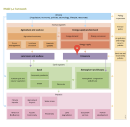
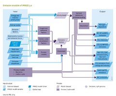
[[Table 5.1]] lists the different sources of emissions | [[Table 5.1]] lists the different sources of emissions included in the IMAGE model. Emissions that are transported in water (nitrate, phosphorus) are discussed in [[Nutrient balances]]. Regarding the approach and spatial detail for modeling gaseous emissions, IMAGE uses four different ways to represent emissions. | ||
* ''World number'' (WRLD). The simplest way to estimate emissions in IMAGE is by using a global estimate from the literature. This approach is used for those natural sources that can not be explicitly modelled. | * ''World number'' (WRLD). The simplest way to estimate emissions in IMAGE is by using a global estimate from the literature. This approach is used for those natural sources that can not be explicitly modelled. | ||
* ''Emission factor method'' (EF). For other sources in IMAGE, past and future developments in anthropogenic emissions are estimated on the basis of projected changes in relevant economic activities and the emissions per unit of activity (emission factor) ([[Figure 5.1]]). | * ''Emission factor method'' (EF). For other sources in IMAGE, past and future developments in anthropogenic emissions are estimated on the basis of projected changes in relevant economic activities and the emissions per unit of activity (emission factor) ([[Figure 5.1]]). | ||
| Line 8: | Line 8: | ||
The equation for this emission factor approach is as follows: | The equation for this emission factor approach is as follows: | ||
{{FormulaAndTableTemplate|Formula1_E}} | {{FormulaAndTableTemplate|Formula1_E}} | ||
where Emission is the emission of the specific gas; Activity is the Energy input or agricultural activity, r is the index for region, i index for further specification (sector, energy carrier), EF-base is the emission factor in the baseline and AF is the abatement factor, i.e. the reduction of the baseline emission factor as a result of climate policy. The emission factors are time-dependent, representing changes in technology and air pollution control policies. | where Emission is the emission of the specific gas; Activity is the Energy input or agricultural activity, r is the index for region, i index for further specification (sector, energy carrier), EF-base is the emission factor in the baseline and AF is the abatement factor, i.e. the reduction of the baseline emission factor as a result of climate policy. The emission factors are time-dependent, representing changes in technology and air pollution control policies. | ||
The emission factor approach is used to calculate energy emissions and several land-use related emissions. Following | The emission factor approach is used to calculate energy emissions and several land-use related emissions. Following the equation above, there is a direct relation between the level of economic activity and emission level. Also shifts in economic activity (e.g. use of natural gas instead of coal) may influence the total emissions. Finally, emissions can change as result of changes in the emission factors (EF) or climate policy (AF). Some generic rules are used to describe the changes of emissions over time (see further). The abatement factor (AF) are determined in the climate policy model [[FAIR model|FAIR]] (see [[Climate policy]]). The emission factor approach has some limitations, most importantly that is limited in capturing the consequences of specific emission control technology (or management action) for multiple species (either synergies or trade-offs). | ||
* ''Emission factor method with spatial distribution'' (GEF) represents a special case of the EF method where a proxy distribution is used to present gridded emissions. This is done for a number of sources, for example emissions from animals ([[Table 5.1]]). | * ''Emission factor method with spatial distribution'' (GEF) represents a special case of the EF method where a proxy distribution is used to present gridded emissions. This is done for a number of sources, for example emissions from animals ([[Table 5.1]]). | ||
| Line 21: | Line 20: | ||
==Emissions from energy production and use== | ==Emissions from energy production and use== | ||
Emission factors (EFs) ( | Emission factors (EFs) (see the equation above) are used to estimate emissions from the various energy-related sources ([[Table 5.2]]). In general, the so-called Tier 1 approach from IPCC guidelines ([[IPCC, 2006]]) is used. In the energy system, emissions are calculated by multiplying energy use fluxes with time-dependent emission factors. Changes in the emission factors represent technological improvements and end of-pipe control techniques, fuel specification standards for transport, clean-coal technologies in industry, etc. | ||
The emission factors are calibrated for the historical period on the basis of the [[EDGAR database|EDGAR emission model]] as described by [[Braspenning Radu et al., 2012]]. The calibration to the EDGAR database is not always straightforward due to differences in aggregation level. The general rule is to use weighted average emission factors in the case of aggregation. However, in those cases in which this results in incomprehensible emission factors (in particular when large differences exists between the emission factors for the underlying technologies) specific emission factors were chosen. | The emission factors are calibrated for the historical period on the basis of the [[EDGAR database|EDGAR emission model]] as described by [[Braspenning Radu et al., 2012]]. The calibration to the EDGAR database is not always straightforward due to differences in aggregation level. The general rule is to use weighted average emission factors in the case of aggregation. However, in those cases in which this results in incomprehensible emission factors (in particular when large differences exists between the emission factors for the underlying technologies) specific emission factors were chosen. | ||
| Line 47: | Line 46: | ||
The CO2 exchange between terrestrial ecosystems and the atmosphere computed by the LPJ model is described in [[Natural vegetation and carbon cycle]]. The land-use emissions model focuses on emissions of other important gases, including greenhouse gases (CH4, N2O), ozone precursors (NOx, CO, VOC), acidifying compounds (SO2, NH3) and aerosols (SO2, NO3, BC, OC). | The CO2 exchange between terrestrial ecosystems and the atmosphere computed by the LPJ model is described in [[Natural vegetation and carbon cycle]]. The land-use emissions model focuses on emissions of other important gases, including greenhouse gases (CH4, N2O), ozone precursors (NOx, CO, VOC), acidifying compounds (SO2, NH3) and aerosols (SO2, NO3, BC, OC). | ||
For many sources, the emission factor approach ( | For many sources, the emission factor approach (see formula 1.) is used ([[Table 5.2]]). For anthropogenic sources, the emission factors are from the EDGAR database, with time-dependent values for historical years. During the scenario period, most emission factors are constant, except for explicit climate abatement policies (see below). However, there are some important exceptions. Atmospheric N emissions are modeled in a detailed way (see below), and in several other cases, the emission factor depends on the assumptions described in other parts of IMAGE. For example, CH4 emissions from nondairy and dairy cattle are calculated on the basis of the energy requirement and feed type (see [[Livestock]]). High-quality feed such as concentrates from feed crops have a lower CH4 emission factor than feeds with lower protein and higher contents of components with lower digestibility. This implies that when the feed conversion ratio changes, the CH4 emission will automatically change as well. Feed conversion ratios are prescribed, or are calculated on the basis of the animal productivity. | ||
Constant emission factors may lead to decreasing emissions per unit of product, for example when the emission factor is specified on a per head basis. An increasing production per head may then lead to a decreasing emission per unit of product. An example is the constant CH4 emission from animal waste per animal, which leads to decreasing emissions per unit of meat or milk when the production per animal increases. | Constant emission factors may lead to decreasing emissions per unit of product, for example when the emission factor is specified on a per head basis. An increasing production per head may then lead to a decreasing emission per unit of product. An example is the constant CH4 emission from animal waste per animal, which leads to decreasing emissions per unit of meat or milk when the production per animal increases. | ||
Revision as of 15:08, 15 January 2014
Parts of Emissions/Description
| Component is implemented in: |
Components:and
|
| Projects/Applications |
| Models/Databases |
| Key publications |
| References |
|