Emissions/Description: Difference between revisions
Jump to navigation
Jump to search
No edit summary |
No edit summary |
||
| Line 51: | Line 51: | ||
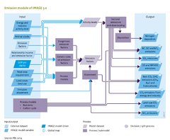
The methodology for EKC scenario development applied in the energy model is based on two types of variables: income thresholds (2–3 steps); and gas- and sector-dependent reduction targets for these income levels. The income thresholds are set to historical points: the average {{abbrTemplate|OECD}} income at which air pollution control policies were introduced in these countries; and current income level in OECD countries. The model assumes that emission factors will start to decline in developing countries, when they reach the first income threshold, reflecting more efficient and cleaner technology. It also assumes that when developing countries reach the second income threshold, the emission factors will be equal to the average level in OECD regions. Beyond this income level, the model assumes further reductions, slowly converging to the minimum emission factor in OECD regions by 2030, according to projections made by {{abbrTemplate|IIASA}} under current legislation (current abatement plans). The IMAGE rules act at the level of regions, this could be seen as a limitation, but as international agreements lead countries to act as a group, this may not be an important limitation. | The methodology for EKC scenario development applied in the energy model is based on two types of variables: income thresholds (2–3 steps); and gas- and sector-dependent reduction targets for these income levels. The income thresholds are set to historical points: the average {{abbrTemplate|OECD}} income at which air pollution control policies were introduced in these countries; and current income level in OECD countries. The model assumes that emission factors will start to decline in developing countries, when they reach the first income threshold, reflecting more efficient and cleaner technology. It also assumes that when developing countries reach the second income threshold, the emission factors will be equal to the average level in OECD regions. Beyond this income level, the model assumes further reductions, slowly converging to the minimum emission factor in OECD regions by 2030, according to projections made by {{abbrTemplate|IIASA}} under current legislation (current abatement plans). The IMAGE rules act at the level of regions, this could be seen as a limitation, but as international agreements lead countries to act as a group, this may not be an important limitation. | ||
Emissions from industrial processes | ===Emissions from industrial processes=== | ||
For the industry sector, the energy model includes three categories: | For the industry sector, the energy model includes three categories: | ||
# Cement and steel production. IMAGE-TIMER includes detailed demand models for these commodities (Component [[Energy supply and demand]]). Similar to those from energy use, emissions are calculated by multiplying the activity levels to exogenously set emission factors. | |||
# Other industrial activities. Activity levels are formulated as a regional function of industry value added, and include copper production and production of solvents. Emissions are also calculated by multiplying the activity levels by the emission factors. | |||
# For halogenated gases, the approach used was developed by Harnisch et al. ([[Harnisch et al., 2009|2009]]), which derived relationships with income for the main uses of halogenated gases (HFCs, PFCs, SF6). In the actual use of the model, slightly updated parameters are used to better represent the projections as presented by Velders et al. ([[Velders et al., 2009|2009]]). The marginal abatement cost curve per gas still follows the methodology described by Harnisch et al. ([[Harnisch et al., 2009|2009]]). | |||
Land-use related emissions | Land-use related emissions | ||
CO2 exchanges between terrestrial ecosystems and the atmosphere computed by the LPJ model are described in Section 6.1. The land-use emissions model focuses on emissions of other compounds, including greenhouse gases (CH4, N2O), ozone precursors (NOx, CO, NMVOC), acidifying compounds (SO2, NH3) and aerosols (SO2, NO3, BC, OC). | CO2 exchanges between terrestrial ecosystems and the atmosphere computed by the LPJ model are described in Section 6.1. The land-use emissions model focuses on emissions of other compounds, including greenhouse gases (CH4, N2O), ozone precursors (NOx, CO, NMVOC), acidifying compounds (SO2, NH3) and aerosols (SO2, NO3, BC, OC). | ||
Revision as of 10:12, 21 May 2014
Parts of Emissions/Description
| Component is implemented in: |
Components:and
|
| Projects/Applications |
| Models/Databases |
| Key publications |
| References |
|
