Energy conversion/Description: Difference between revisions
No edit summary |
(Added hydrogen sector improvements) |
||
| (81 intermediate revisions by 8 users not shown) | |||
| Line 1: | Line 1: | ||
{{ComponentDescriptionTemplate | {{ComponentDescriptionTemplate | ||
|Reference=Hoogwijk, 2004; Van Vuuren, 2007; Hendriks et al., 2004b; Van Ruijven et al., 2007; Ueckerdt et al., 2016; Gernaat et al., 2014; Köberle et al., 2015; De Boer and Van Vuuren, 2017; | |||
|Reference=Hoogwijk, 2004; Van Vuuren, 2007; Hendriks et al., 2004b; Van Ruijven et al., 2007; | }} | ||
<div class="page_standard"> | |||
[[TIMER model|TIMER]] includes two main energy conversion modules: Electric power generation and hydrogen generation. Below, electric power generation is described in detail. In addition, the key characteristics of the hydrogen generation model, which follows a similar structure, are presented. | |||
===Electric power generation=== | |||
In TIMER, electricity can be generated by 32 technologies. These include the VRE sources solar utility scale photovoltaic (PV), residential photovoltaics (RPV), concentrated solar power (CSP), ocean wave power and onshore and offshore wind power. Other technology types are natural gas-, coal-, biomass- and oil-fired power plants. These power plants come in multiple variations: conventional, combined cycle, carbon capture and storage (CCS) and combined heat and power (CHP). The electricity sector in TIMER also describes the use of nuclear, other renewables (mainly geothermal power) and hydroelectric power. A recent addition is the use of hydrogen for electricity and heat generation. ([[De Boer and Van Vuuren, 2017]]) | |||
As shown in the [[Flowchart Energy conversion|flowchart]], two key elements of the electric power generation are the investment strategy and the operational strategy in the sector. A challenge in simulating electricity production in an aggregated model is that in reality electricity production depends on a range of complex factors, related to costs, reliance, and technology ramp rates. Modelling these factors requires a high level of detail and thus IAMs, such as TIMER, concentrate on introducing a set of simplified, meta relationships ([[Hoogwijk, 2004]]; [[Van Vuuren, 2007]]; [[De Boer and Van Vuuren, 2017]]). | |||
As shown in the | |||
==Total demand for new capacity== | ====Total demand for new capacity==== | ||
The | <div class="version changev31"> | ||
The electricity generation capacity required to meet the demand per region is based on a forecast of the maximum annual electricity demand plus a reserve margin. The reserve margin consists of a general reserve margin of 10-20% on peak demand plus a compensation for imperfect capacity credits (the reliability of a plant type to supply power during the peak hours) of existing capacity. The maximum annual demand is calculated on the basis of an assumed shape of the load duration curve (LDC) and the gross electricity demand. The latter comprises the net electricity demand from the end-use sectors plus electricity trade and transmission losses. An LDC shows the distribution of load over a certain timespan in a downward form. The peak load is plotted to the left of the LDC and the lowest load is plotted to the right. The shape of the LDC is based on work by Ueckerdt et al. ([[Ueckerdt et al., 2016|2016]]), who derived regional normalized residual LDCs (RLDC) for different solar and wind shares, including the application of optimized electricity storage. | |||
The final demand for new generation capacity is equal to the difference between the required and existing capacity. Power capacity is assumed to be replaced at the end of its lifetime, which varies from 25 to 80 years, depending on the technology. | |||
Capacity can also be decommissioned before the end of the technical lifetime. This so-called early retirement can occur if the operation of the capacity has become relatively expensive compared to the operation and construction of new capacity. The operational costs include fixed O&M, variable O&M, fuel and CCS costs. Capacity will not be retired early if the capacity has a backup role, characterized by a low load factor resulting in low operational costs and carbon emissions. ([[De Boer and Van Vuuren, 2017]]) | |||
</div> | |||
== | ====Decisions to invest in specific options ==== | ||
In the model, the decision to invest in generation technologies is based on the levelized cost of electricity (LCOE; in USD/kWhe) produced per technology, using a multinomial logit equation that assigns larger market shares to the lower cost options. | |||
An important variable used in determining the LCOE is the expected amount of electricity generated. Often, the LCOEs of technologies are compared at maximum full load hours. However, only a limited share of the installed capacity will actually generate electricity at full load. This effect is captured in a heuristic: different load bands have been introduced to link the investment decision to expected dispatch. The different load bands are distributed among the LDC, resulting in a load factor for each load band. The inclusion of different load factors for each load band means that less capital-intensive technologies are attractive to use for lower load factor load bands. These are likely to be gas-fired peaker plants. For load bands with higher load factors, the electricity submodule chooses technologies with lower operational costs. These are likely to be base load plants, such as coal-fired or nuclear power plants. VRE load factors per load band are derived from the marginal load band contributions resulting from the RLDC. A system with more VRE sources will result in lower residual load factors and therefore in a higher demand for peak or mid load technologies. ([[De Boer and Van Vuuren, 2017]]) | |||
The standard costs of each option can be broken down into several categories: investment or capital cost; fuel cost; fixed and variable operational and maintenance costs; construction costs; and carbon capture and storage costs. | |||
* The capital costs of power generating technologies can be exogenously described, but they can also develop as a result of endogenous learning mechanisms explained [[Technical learning|here]]. For the endogenous method, technologies are split up in different cost components. These components have individual learning characteristics, like learning rate, floor costs and start costs. However, spillovers are possible between technologies and regions. Technology spillovers occur when technologies share a component. | |||
* Fuel cost result from the supply modules described [[Energy supply|here]]. | |||
* Fixed and variable operation and maintenance costs develop according to the same principles as the capital costs | |||
* Construction costs result from interest paid during construction. Construction times vary among the technologies. | |||
* More information on carbon capture and storage cost can be found [[Carbon capture and storage|here]]. | |||
Also, additional costs are distinguished: backup costs; curtailment costs; VRE load factor decline; storage costs; and transmission and distribution costs. | |||
* Backup costs have been added to represent the additional costs required in order to meet the capacity and energy production requirements of a load band. Backup costs are usually higher for technologies with low capacity credits. Backup costs include all standard cost components for the chosen backup technology. This backup capacity is installed together with regular investments in load bands | |||
* Curtailment costs are only relevant for VRE technologies and CHP. Curtailments occur when the supply exceeds the demand. The degree to which curtailment occurs depends on VRE share, storage use and the regional correlation between electricity demand and VRE or CHP supply. Curtailment influences the LCOE by reducing the potential amount of electricity that could be generated. | |||
* Load factor reduction results from the utilisation of resource sites with less favourable environmental conditions, such as lower wind speeds, lower water discharge or less solar irradiation. This results in a lower potential load influencing the LCOE by reducing the potential electricity generation. The development of load factor reduction is captured in cost supply curves. For more information on the TIMER cost supply curves see: Hoogwijk ([[Hoogwijk, 2004|2004]]), Gernaat et al., ([[Gernaat et al., 2014|2014]]), Koberle et al., ([[Köberle et al., 2015|2015]]) and Gernaat et al., (<nowiki>[[2018]]</nowiki>) | |||
* Storage use has been optimised in the RLDC data set. For more information on storage use, see Ueckerdt et al. (n.d.). | |||
* Transmission and distribution costs are simulated by adding a fixed relationship between the amount of capacity and the required amount of transmission and distribution capital. VRE cost supply curves contain additional transmission costs resulting from distance between VRE potential and demand centres. | |||
The exceptions are ''other renewables'' and CHP. ''Other renewables'' are exogenously prescribed, because of a lack of available data. The demand for CHP capacity is heat demand driven. ([[De Boer and Van Vuuren, 2017]]) | |||
Finally, in the equations, some constraints are added to account for limitations in supply, for example restrictions on biomass availability. For a more detailed description on electricity sector investments in TIMER, see [[De Boer and Van Vuuren, 2017]]). | |||
====Operational strategy==== | |||
The demand for electricity is met by the installed capacity of power plants. The available capacity is used according to the merit order of the different types of plants; technologies with the lowest variable costs are dispatched first, followed by other technologies based on an ascending order of variable costs. This results in a cost-optimal dispatch of technologies. The dispatch of VRE is described by the RLDC dataset. CHP dispatch is distributed based on monthly heating degree days. Within each month, the CHP load stays constant. Hydropower has a monthly dispatch potential. This limited availability of hydropower is distributed so that so that it creates most system benefits. Generally, this has a peak shaving effect on residual demand for electricity. | |||
==Hydrogen generation | ===Hydrogen generation=== | ||
The structure of the hydrogen | The structure of the hydrogen generation submodule is similar to that for electric power generation ([[Van Ruijven et al., 2007]]) but with following differences: | ||
#There are 17 supply options for hydrogen production: | |||
without carbon capture and storage (8 plants) | #* coal, oil, natural gas and bioenergy, with and without carbon capture and storage (8 plants); | ||
* | #* grid electrolysis: | ||
#** a technology producing hydrogen at a constant rate resulting in a baseload electricity demand | |||
#** a technology producing hydrogen just from cheap VRE curtailments, reducing curtailment levels in the electricity sector | |||
#*direct renewable electrolysis: | |||
#** combining solar PV, CSP, onshore wind and offshore wind technologies directly with an electrolyser | |||
#** avoids electricity grid costs | |||
#** shared technological learning with electricity production technologies | |||
#* small scale technologies at low hydrogen demand levels: | |||
#** small methane reform plant | |||
#** small scale electrolyser | |||
#No description of preferences for different power plants is taken into account in the operational strategy. The load factor for each option equals the total production divided by the capacity for each region. The direct electrolysis technologies and the curtailment electrolyser are exceptions: here the load factor is limited by the supply technology | |||
#Intermittence does not play an important role because hydrogen can be stored to some degree. Thus, there are no equations simulating system integration. | |||
#Hydrogen can be traded. A trade model is added, similar to those for fossil fuels described in [[Energy supply]]. | |||
< | See the additional info on [[Grid and infrastructure]]. | ||
</div> | |||
Latest revision as of 11:37, 3 November 2022
Parts of Energy conversion/Description
| Component is implemented in: |
|
| Related IMAGE components |
| Projects/Applications |
| Models/Databases |
| Key publications |
| References |
Model description of Energy conversion
TIMER includes two main energy conversion modules: Electric power generation and hydrogen generation. Below, electric power generation is described in detail. In addition, the key characteristics of the hydrogen generation model, which follows a similar structure, are presented.
Electric power generation
In TIMER, electricity can be generated by 32 technologies. These include the VRE sources solar utility scale photovoltaic (PV), residential photovoltaics (RPV), concentrated solar power (CSP), ocean wave power and onshore and offshore wind power. Other technology types are natural gas-, coal-, biomass- and oil-fired power plants. These power plants come in multiple variations: conventional, combined cycle, carbon capture and storage (CCS) and combined heat and power (CHP). The electricity sector in TIMER also describes the use of nuclear, other renewables (mainly geothermal power) and hydroelectric power. A recent addition is the use of hydrogen for electricity and heat generation. (De Boer and Van Vuuren, 2017)
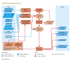
As shown in the flowchart, two key elements of the electric power generation are the investment strategy and the operational strategy in the sector. A challenge in simulating electricity production in an aggregated model is that in reality electricity production depends on a range of complex factors, related to costs, reliance, and technology ramp rates. Modelling these factors requires a high level of detail and thus IAMs, such as TIMER, concentrate on introducing a set of simplified, meta relationships (Hoogwijk, 2004; Van Vuuren, 2007; De Boer and Van Vuuren, 2017).
Total demand for new capacity
The electricity generation capacity required to meet the demand per region is based on a forecast of the maximum annual electricity demand plus a reserve margin. The reserve margin consists of a general reserve margin of 10-20% on peak demand plus a compensation for imperfect capacity credits (the reliability of a plant type to supply power during the peak hours) of existing capacity. The maximum annual demand is calculated on the basis of an assumed shape of the load duration curve (LDC) and the gross electricity demand. The latter comprises the net electricity demand from the end-use sectors plus electricity trade and transmission losses. An LDC shows the distribution of load over a certain timespan in a downward form. The peak load is plotted to the left of the LDC and the lowest load is plotted to the right. The shape of the LDC is based on work by Ueckerdt et al. (2016), who derived regional normalized residual LDCs (RLDC) for different solar and wind shares, including the application of optimized electricity storage.
The final demand for new generation capacity is equal to the difference between the required and existing capacity. Power capacity is assumed to be replaced at the end of its lifetime, which varies from 25 to 80 years, depending on the technology.
Capacity can also be decommissioned before the end of the technical lifetime. This so-called early retirement can occur if the operation of the capacity has become relatively expensive compared to the operation and construction of new capacity. The operational costs include fixed O&M, variable O&M, fuel and CCS costs. Capacity will not be retired early if the capacity has a backup role, characterized by a low load factor resulting in low operational costs and carbon emissions. (De Boer and Van Vuuren, 2017)
Decisions to invest in specific options
In the model, the decision to invest in generation technologies is based on the levelized cost of electricity (LCOE; in USD/kWhe) produced per technology, using a multinomial logit equation that assigns larger market shares to the lower cost options.
An important variable used in determining the LCOE is the expected amount of electricity generated. Often, the LCOEs of technologies are compared at maximum full load hours. However, only a limited share of the installed capacity will actually generate electricity at full load. This effect is captured in a heuristic: different load bands have been introduced to link the investment decision to expected dispatch. The different load bands are distributed among the LDC, resulting in a load factor for each load band. The inclusion of different load factors for each load band means that less capital-intensive technologies are attractive to use for lower load factor load bands. These are likely to be gas-fired peaker plants. For load bands with higher load factors, the electricity submodule chooses technologies with lower operational costs. These are likely to be base load plants, such as coal-fired or nuclear power plants. VRE load factors per load band are derived from the marginal load band contributions resulting from the RLDC. A system with more VRE sources will result in lower residual load factors and therefore in a higher demand for peak or mid load technologies. (De Boer and Van Vuuren, 2017)
The standard costs of each option can be broken down into several categories: investment or capital cost; fuel cost; fixed and variable operational and maintenance costs; construction costs; and carbon capture and storage costs.
- The capital costs of power generating technologies can be exogenously described, but they can also develop as a result of endogenous learning mechanisms explained here. For the endogenous method, technologies are split up in different cost components. These components have individual learning characteristics, like learning rate, floor costs and start costs. However, spillovers are possible between technologies and regions. Technology spillovers occur when technologies share a component.
- Fuel cost result from the supply modules described here.
- Fixed and variable operation and maintenance costs develop according to the same principles as the capital costs
- Construction costs result from interest paid during construction. Construction times vary among the technologies.
- More information on carbon capture and storage cost can be found here.
Also, additional costs are distinguished: backup costs; curtailment costs; VRE load factor decline; storage costs; and transmission and distribution costs.
- Backup costs have been added to represent the additional costs required in order to meet the capacity and energy production requirements of a load band. Backup costs are usually higher for technologies with low capacity credits. Backup costs include all standard cost components for the chosen backup technology. This backup capacity is installed together with regular investments in load bands
- Curtailment costs are only relevant for VRE technologies and CHP. Curtailments occur when the supply exceeds the demand. The degree to which curtailment occurs depends on VRE share, storage use and the regional correlation between electricity demand and VRE or CHP supply. Curtailment influences the LCOE by reducing the potential amount of electricity that could be generated.
- Load factor reduction results from the utilisation of resource sites with less favourable environmental conditions, such as lower wind speeds, lower water discharge or less solar irradiation. This results in a lower potential load influencing the LCOE by reducing the potential electricity generation. The development of load factor reduction is captured in cost supply curves. For more information on the TIMER cost supply curves see: Hoogwijk (2004), Gernaat et al., (2014), Koberle et al., (2015) and Gernaat et al., ([[2018]])
- Storage use has been optimised in the RLDC data set. For more information on storage use, see Ueckerdt et al. (n.d.).
- Transmission and distribution costs are simulated by adding a fixed relationship between the amount of capacity and the required amount of transmission and distribution capital. VRE cost supply curves contain additional transmission costs resulting from distance between VRE potential and demand centres.
The exceptions are other renewables and CHP. Other renewables are exogenously prescribed, because of a lack of available data. The demand for CHP capacity is heat demand driven. (De Boer and Van Vuuren, 2017)
Finally, in the equations, some constraints are added to account for limitations in supply, for example restrictions on biomass availability. For a more detailed description on electricity sector investments in TIMER, see De Boer and Van Vuuren, 2017).
Operational strategy
The demand for electricity is met by the installed capacity of power plants. The available capacity is used according to the merit order of the different types of plants; technologies with the lowest variable costs are dispatched first, followed by other technologies based on an ascending order of variable costs. This results in a cost-optimal dispatch of technologies. The dispatch of VRE is described by the RLDC dataset. CHP dispatch is distributed based on monthly heating degree days. Within each month, the CHP load stays constant. Hydropower has a monthly dispatch potential. This limited availability of hydropower is distributed so that so that it creates most system benefits. Generally, this has a peak shaving effect on residual demand for electricity.
Hydrogen generation
The structure of the hydrogen generation submodule is similar to that for electric power generation (Van Ruijven et al., 2007) but with following differences:
- There are 17 supply options for hydrogen production:
- coal, oil, natural gas and bioenergy, with and without carbon capture and storage (8 plants);
- grid electrolysis:
- a technology producing hydrogen at a constant rate resulting in a baseload electricity demand
- a technology producing hydrogen just from cheap VRE curtailments, reducing curtailment levels in the electricity sector
- direct renewable electrolysis:
- combining solar PV, CSP, onshore wind and offshore wind technologies directly with an electrolyser
- avoids electricity grid costs
- shared technological learning with electricity production technologies
- small scale technologies at low hydrogen demand levels:
- small methane reform plant
- small scale electrolyser
- No description of preferences for different power plants is taken into account in the operational strategy. The load factor for each option equals the total production divided by the capacity for each region. The direct electrolysis technologies and the curtailment electrolyser are exceptions: here the load factor is limited by the supply technology
- Intermittence does not play an important role because hydrogen can be stored to some degree. Thus, there are no equations simulating system integration.
- Hydrogen can be traded. A trade model is added, similar to those for fossil fuels described in Energy supply.
See the additional info on Grid and infrastructure.