Energy conversion/Description: Difference between revisions
Jump to navigation
Jump to search
No edit summary |
No edit summary |
||
| Line 1: | Line 1: | ||
{{ComponentDescriptionTemplate | {{ComponentDescriptionTemplate | ||
|Status=On hold | |Status=On hold | ||
|Reference=Hoogwijk, 2004; Van Vuuren, 2007; Hendriks et al., 2004b; Van Ruijven et al., 2007; | |Reference=Hoogwijk, 2004; Van Vuuren, 2007; Hendriks et al., 2004b; Van Ruijven et al., 2007; | ||
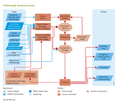
|Description=The [[TIMER model]] includes two energy conversion submodels: the electric power generation model and the hydrogen generation model. Here, the focus is on a description of the electric power generation model (The flowdiagram on the right also shows only the electricity model). The hydrogen model follows a similar structure, and its key characteristics are briefly discussed in this Section. | |Description=The [[TIMER model]] includes two energy conversion submodels: the electric power generation model and the hydrogen generation model. Here, the focus is on a description of the electric power generation model (The flowdiagram on the right also shows only the electricity model). The hydrogen model follows a similar structure, and its key characteristics are briefly discussed in this Section. | ||
| Line 34: | Line 34: | ||
The costs of solar and wind power are the model determinedby learning and depletion dynamics. For renewable energy, costs relate to capital, O&M and system integration. The capital costs mostly relate to learning and depletion processes (learning is depicted in learning curves, ******see Box X; depletion is shown in cost–supply curves). | The costs of solar and wind power are the model determinedby learning and depletion dynamics. For renewable energy, costs relate to capital, O&M and system integration. The capital costs mostly relate to learning and depletion processes (learning is depicted in learning curves, ******see Box X; depletion is shown in cost–supply curves). | ||
The additional system integration costs relate to | The additional system integration costs relate to | ||
# discarded electricity in cases where production exceeds demand and the overcapacity cannot be used within the system, | |||
# back-up capacity | |||
# additional, required spinning reserve. | |||
The two last items are needed to avoid loss of power if the supply of wind or solar power suddenly drops, enabling a power scale up in a relatively short time, in power stations operating below maximum capacity ([[Hoogwijk, 2004]]). | |||
*To determine discarded electricity, the model makes a comparison between 10 different points on the load-demand curve, at the overlap between demand and supply. For both wind and solar power, a typical load–supply curve is assumed (see [[Hoogwijk, 2004]]). If supply exceeds demand, the overcapacity in electricity is assumed to be discarded, resulting in higher production costs. | *To determine discarded electricity, the model makes a comparison between 10 different points on the load-demand curve, at the overlap between demand and supply. For both wind and solar power, a typical load–supply curve is assumed (see [[Hoogwijk, 2004]]). If supply exceeds demand, the overcapacity in electricity is assumed to be discarded, resulting in higher production costs. | ||
*Because wind and solar power supply is intermittent (i.e. it varies and therefore is not reliable), the model assumes that so-called back-up capacity needs to be installed. For the first 5% penetration of the intermittent capacity, it is assumed that no-back is required. However, for higher levels of penetration, the effective capacity (i.e. degree to which operators can rely on plants producing at a particular moment in time) of intermittent resources is assumed to decrease (referred to as the capacity factor). This decrease leads to the need of back-up power(by low-cost options, such as gas turbines), the costs of which are allocated to the intermittent source. | *Because wind and solar power supply is intermittent (i.e. it varies and therefore is not reliable), the model assumes that so-called back-up capacity needs to be installed. For the first 5% penetration of the intermittent capacity, it is assumed that no-back is required. However, for higher levels of penetration, the effective capacity (i.e. degree to which operators can rely on plants producing at a particular moment in time) of intermittent resources is assumed to decrease (referred to as the capacity factor). This decrease leads to the need of back-up power(by low-cost options, such as gas turbines), the costs of which are allocated to the intermittent source. | ||
| Line 40: | Line 44: | ||
==Nuclear power== | ==Nuclear power== | ||
For nuclear power, the costs also consists of capital, O&M and nuclear fuel costs. Similar to the renewable energy options, technology improvement nuclear power is described via a learning curve (so costs decrease with cumulative installed capacity). At the same time, fuel costs increase as a function of depletion. Fuel costs are determined on the basis of the estimated extraction costs of uranium and thorium resources, as is described in the component [[Energy supply]] . A small trade model for these fission fuels is included. | For nuclear power, the costs also consists of capital, O&M and nuclear fuel costs. Similar to the renewable energy options, technology improvement nuclear power is described via a learning curve (so costs decrease with cumulative installed capacity). At the same time, fuel costs increase as a function of depletion. Fuel costs are determined on the basis of the estimated extraction costs of uranium and thorium resources, as is described in the component [[Energy supply]]. A small trade model for these fission fuels is included. | ||
==Hydrogen generation model== | ==Hydrogen generation model== | ||
Revision as of 15:11, 9 December 2013
Parts of Energy conversion/Description
| Component is implemented in: |
|
| Related IMAGE components |
| Projects/Applications |
| Models/Databases |
| Key publications |
| References |