Agricultural economy/Description: Difference between revisions
Jump to navigation
Jump to search
m (Text replace - "|Status=On hold" to "") |
No edit summary |
||
| Line 1: | Line 1: | ||
{{ComponentDescriptionTemplate | {{ComponentDescriptionTemplate | ||
|Reference=Hertel, 1997; Britz, 2003; Armington, 1969; Huang et al., 2004; Helming et al., 2010; Banse et al., 2008; Bruinsma, 2003; | |Reference=Hertel, 1997; Britz, 2003; Armington, 1969; Huang et al., 2004; Helming et al., 2010; Banse et al., 2008; Bruinsma, 2003; | ||
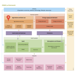
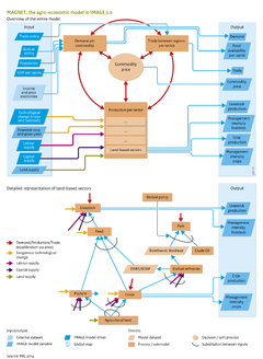
|Description=The [[MAGNET model]] ([[Woltjer et al., 2011]]) is based on the standard [[GTAP model]] ([[Hertel, 1997]]), which is a multi-regional, static, applied computable general equilibrium ([[CGE]]) model based on neoclassical microeconomic theory. Although | |Description=The [[MAGNET model]] ([[Woltjer et al., 2011]]) (Woltjer et al., 2011) is based on the standard [[GTAP model]] ([[Hertel, 1997]]), which is a multi-regional, static, applied computable general equilibrium ([[CGE]]) model based on neoclassical microeconomic theory. Although the model covers the entire economy, there is a special focus on agricultural sectors. It is a further development of GTAP regarding land use, household consumption, livestock, food, feed and energy crop production, and emission reduction from deforestation. | ||
=== Demand and supply === | === Demand and supply === | ||
Household demand for agricultural products is calculated as a function of income, income elasticities, price elasticities, and cross-price elasticities. Income elasticities for agricultural commodities are consistent with [[FAO]] estimates ([[Britz, 2003]]), and dynamically depend on purchasing power parity ([[HasAcronym::ppp]]) corrected [[GDP per capita]]. The supply of all commodities is modelled by an input–output structure that explicitly links the production of goods and services for final consumption via different stages | Household demand for agricultural products is calculated as a function of income, income elasticities, price elasticities, and cross-price elasticities. Income elasticities for agricultural commodities are consistent with with [[FAO]] estimates ([[Britz, 2003]]), and dynamically depend on purchasing power parity ([[HasAcronym::ppp]]) corrected [[GDP per capita]]. The supply of all commodities is modelled by an input–output structure that explicitly links the production of goods and services for final consumption via different processing stages back to primary products (crops and livestock products) and resources. At each production level, input of labour, capital, and intermediate input or resources (e.g., land) can be substituted for one another. For example, labour, capital and land are input factors in crop production, and substitution of these production factors is driven by changes in their relative prices. If the price of one input factor increases, it is substituted by other factors, following the price elasticity of substitution. | ||
=== Regional aggregation and trade === | |||
MAGNET is flexible in its regional aggregation (129 regions). In linking with IMAGE, MAGNET distinguishes individual European countries and 22 large world regions, closely matching the regions in IMAGE (Figure zzz IMAGE regions). Similar to most other CGE models, MAGNET assumes that products traded internationally are differentiated according to country of origin. Thus, domestic and foreign products are not identical, but are imperfect substitutes (Armington assumption; Armington, 1969). (Armington, 1969). | |||
Land use: In addition to the standard GTAP model, MAGNET includes a dynamic land supply function (Van Meijl et al., 2006) (Van Meijl et al., 2006) that accounts for the availability and suitability of land for agricultural use, based on information from IMAGE (see below, and Figure 4.2.1). A nested land-use structure accounts for the differences in substitutability of the various types of land use (Huang et al., 2004; Van Meijl et al., 2006) (Huang et al., 2004; Van Meijl et al., 2006). In addition, the MAGNET model includes international and EU agricultural policies, such as production quota and export\import tariffs (Helming et al., 2010) (Helming et al., 2010) . | |||
Biofuel crops: MAGNET includes ethanol and biodiesel as first-generation biofuels made from wheat, sugar cane, maize, and oilseeds (Banse et al., 2008) (Banse et al., 2008) , and accounts for the use of by-products (DDGS, oilcakes) from biofuel production in the livestock sector. | |||
Livestock: MAGNET distinguishes the livestock commodities of beef and other ruminant meats, dairy cattle (grass- and crop-fed), and a category of other animals (e.g., chickens and pigs) that are primarily crop fed. Modelling the livestock sector includes different feedstuffs, such as feed crops, co-products from biofuels (oil cakes from rapeseed-based biofuel, or distillers grain from wheat-based biofuels), and grass (Woltjer, 2011). Grass may be substituted by feed from crops for ruminants. | |||
Land supply: In MAGNET, land supply is calculated using a land supply curve that relates the area in use for agriculture to the land price (Figure 4.1.1.c ). Total land supply includes all land that is potentially available for agriculture, where crop production is possible under soil and climatic conditions, and where no other restrictions apply such as urban or protected area designations (see also Section 4.2.3). In the IMAGE model, total land supply for each region is obtained from potential crop productivity and land availability on a resolution of 5 by 5 arcminutes. Within this total potential, the land supply curve indicates the price at which additional land is put into use. The supply curve depends on total land supply, current agricultural area, current land price, and the estimated current price elasticity of land supply. Regions differ with regard to the proportion of land in use, and with regard to change in land prices in relation to changes in agricultural land use. In regions where most of the area suitable for agriculture is in use, the price elasticity of land supply is small, with little expansion occurring at high price changes. In contrast, in regions with a large reserve of suitable agricultural land, such as Sub-Saharan Africa and some regions in South America, the price elasticity of land supply is large, with extensive expansion of agricultural land occurring at small price changes. | |||
Reduced land availability: By restricting land supply in IMAGE and MAGNET, the models can assess scenarios with additional protected areas, or reduced emissions from deforestation and forest degradation (REDD). | |||
Intensification of crop and pasture production: Crop and pasture yields in MAGNET may change as a result of the following four processes: | |||
# autonomous technological change (external scenario assumption); | |||
# intensification due to the substitution of production factors (endogenous); | |||
# climate change (from IMAGE); | |||
# change in agricultural area affecting crop yields (such as, decreasing average yields due to expansion into less suitable regions; from IMAGE). | |||
Biophysical yield effects due to climate and area changes are calculated by the IMAGE crop model and communicated to MAGNET. External assumptions on autonomous technological changes are mostly based on FAO projections (Bruinsma, 2013) (Bruinsma, 2003) , which describe per region and commodity, the assumed future changes in yields for a wide range of crop types. In MAGNET, the biophysical yield changes are combined with the autonomous technological change to give the total exogenous yield change. In addition, during the simulation period, MAGNET calculates an endogenous intensification as a result of price-driven substitution between labour, land and capital. In IMAGE, regional yield changes due to autonomous technological change and endogenous intensification according to MAGNET are used in the spatially explicit allocation of land use (Section 4.2.3). | |||
===OLD=== | |||
=== Regional aggregation and trade === | === Regional aggregation and trade === | ||
Revision as of 18:23, 10 February 2014
Parts of Agricultural economy/Description
| Component is implemented in: |
|
| Related IMAGE components |
| Projects/Applications |
| Key publications |
| References |