|
|
| Line 1: |
Line 1: |
| {{ComponentDescriptionTemplate | | {{ComponentPolicyIssueTemplate |
| |Reference=IPCC, 2006; Cofala et al., 2002; Stern, 2003; Smith et al., 2005; Van Ruijven et al., 2008; Carson, 2010; Smith et al., 2011; Bouwman et al., 1993; Velders et al., 2009; Kreileman and Bouwman, 1994; Bouwman et al., 1997; Bouwman et al., 2002a; Velders et al., 2009; Harnisch et al., 2009; Braspenning Radu et al., 2016; | | |Reference=PBL, 2012; Braspenning Radu et al., 2016; |
| }} | | }} |
| <div class="page_standard"> | | <div class="page_standard"> |
| ==Model description of {{ROOTPAGENAME}}== | | ==Baseline developments== |
| ===General approaches===
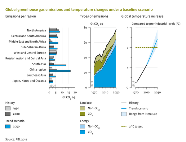
| | In a baseline scenario, most greenhouse gas emissions tend to increase, driven by an increase in underlying activity levels (This is shown in the figure below for a baseline scenario for the [[Roads from Rio+20 (2012) project|Rio+20]] study ([[PBL, 2012]]). For air pollutants, the pattern also depends strongly on the assumptions on air pollution control. In most baseline scenarios, air pollutant emissions tend to decrease, or at least stabilise, in the coming decades as a result of more stringent environmental standards in high and middle income countries. |
| Air pollution emission sources included in IMAGE are listed in [[Emission table]], and emissions transported in water (nitrate, phosphorus) are discussed in Component [[Nutrients]]. In approach and spatial detail, gaseous emissions are represented in IMAGE in four ways:
| |
|
| |
|
| 1) ''World number (W)'' | | {{DisplayPolicyInterventionFigureTemplate|{{#titleparts: {{PAGENAME}}|1}}|Baseline figure}} |
|
| | ==Policy interventions== |
| :The simplest way to estimate emissions in IMAGE is to use global estimates from the literature. This approach is used for natural sources that cannot be modelled explicitly ([[Emission table]]).
| |
|
| |
|
| 2) ''Emission factor (EF)'' | | Policy scenarios present several ways to influence emission of air pollutants ([[Braspenning Radu et al., 2016]]): |
| | * Introduction of climate policy, which leads to systemic changes in the energy system (less combustion) and thus, indirectly to reduced emissions of air pollutants ([[Van Vuuren et al., 2006]]). |
| | * Policy interventions can be mimicked by introducing an alternative formulation of emission factors to the standard formulations ({{abbrTemplate|EKC}}, {{abbrTemplate|CLE}}). For instance, emission factors can be used to deliberately include maximum feasible reduction measures. |
| | * Policies may influence emission levels for several sources, for instance, by reducing consumption of meat products. By improving the efficiency of fertiliser use, emissions of N<sub>2</sub>O, NO and NH<sub>3</sub> can be decreased ([[Van Vuuren et al., 2011b]]). By increasing the amount of feed crops in the cattle rations, CH<sub>4</sub> emissions can be reduced. Production of crop types has a significant influence on emission levels of N<sub>2</sub>O, NO<sub>x</sub> and NH<sub>3</sub> from spreading manure and fertilisers. |
| | * Assumptions related to soil and nutrient management. The major factors are fertiliser type and mode of manure and fertiliser application. Some fertilisers cause higher emissions of N<sub>2</sub>O and NH<sub>3</sub> than others. Incorporating manure into soil lowers emissions compared to broadcasting. |
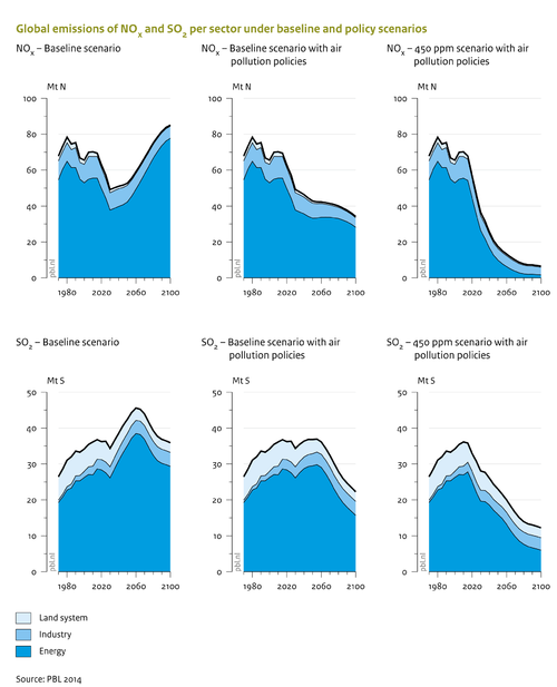
| | The impacts of more ambitious control policies ({{abbrTemplate|CLE}} versus {{abbrTemplate|EKC}}) on SO<sub>2</sub> and NO<sub>x</sub>, emissions, and the influence of climate policy are presented in the figure below. Where climate policy is particularly effective in reducing SO<sub>2</sub> emissions, air pollution control policies are effective in reducing NO<sub>x</sub> emissions. |
|
| |
|
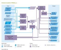
| :Past and future developments in anthropogenic emissions are estimated on the basis of projected changes in activity and emissions per unit of activity (Figure Flowchart).
| | See also the Policy interventions Table below. |
|
| |
|
| :The equation for this emission factor approach is: | | {{DisplayPolicyInterventionFigureTemplate|{{#titleparts: {{PAGENAME}}|1}}|Policy intervention figure}} |
| ::<math>Emission = Activity_{r,i} * EFbase_{r,i} * AF_{r,i}</math> (Equation 1)
| |
| :where:
| |
| :* <math>Emission</math> is the emission of the specific gas or aerosol;
| |
| :* <math>Activity</math> is the energy input or agricultural activity; r is the index for region;
| |
| :* <math>i</math> is the index for further specification (sector, energy carrier);
| |
| :* <math>EFbase</math> is the emission factor in the baseline;
| |
| :* <math>AF</math> is the abatement factor (reduction in the baseline emission factor as a result of climate policy).
| |
| :The emission factors are time-dependent, representing changes in technology and air pollution control and climate mitigation policies.
| |
|
| |
|
| :The emission factor is used to calculate energy and industry emissions, and agriculture, waste and land-use related emissions. Following Equation 1, there is a direct relationship between level of economic activity and emission level. Shifts in economic activity (e.g., use of natural gas instead of coal) may influence total emissions. Finally, emissions can change as a result of changes in emission factors (EF) and climate policy (AF).
| | {{PIEffectOnComponentTemplate }} |
| :Some generic rules are used in describing changes in emissions over time (see further). The abatement factor (AF) is determined in the climate policy model FAIR (see Component [[Climate policy]]). The emission factor approach has some limitations, the most important of which is capturing the consequences of specific emission control technology (or management action) for multiple gas species, either synergies or trade-offs.
| |
| | |
| 3) ''Gridded emission factor with spatial distribution (GEF)''
| |
| | |
| :GEF is a special case of the EF method, where a proxy distribution is used to present gridded emissions. This is done for a number of sources, such as emissions from livestock ([[Emission table]]).
| |
| | |
| 4) ''Gridded process model (GPM)''
| |
| :Land-use related emissions of NH<sub>3</sub>, N<sub>2</sub>O and NO are calculated with grid-specific models (Figure Flowchart). The models included in IMAGE are simple regression models that generate an emission factor (Figure Flowchart). For comparison with other models, IMAGE also includes the N<sub>2</sub>O methodology generally proposed by {{abbrTemplate|IPCC}} ([[IPCC, 2006]]).
| |
| | |
| The approaches used to calculate emissions from energy production and use, industrial processes and land-use related sources are discussed in more detail below.
| |
| | |
| ===Emissions from energy production and use===
| |
| Emission factors ([[#General approaches|Equation 1]]) are used for estimating emissions from the energy-related sources ([[Emission table]]). In general, the Tier 1 approach from IPCC guidelines ([[IPCC, 2006]]) is used. In the energy system, emissions are calculated by multiplying energy use fluxes by time-dependent emission factors. Changes in emission factors represent, for example, technology improvements and end-of-pipe control techniques, fuel emission standards for transport, and clean-coal technologies in industry.
| |
| | |
| The emission factors for the historical period for the energy system and industrial processes are calibrated with the EDGAR emission model described by Braspenning Radu et al. ([[Braspenning Radu et al., 2016]]). Calibration to the EDGAR database is not always straightforward because of differences in aggregation level. The general rule is to use weighted average emission factors for aggregation. However, where this results in incomprehensible emission factors (in particular, large differences between the emission factors for the underlying technologies), specific emission factors were chosen.
| |
| | |
| Future emission factors are based on the following rules:
| |
| | |
| * Emission factors can follow an exogenous scenario, which can be based on the storyline of the scenario. In some cases, exogenous emission factor scenarios are used, such as the Current Legislation Scenario ({{abbrTemplate|CLE}}) developed by IIASA (for instance, Cofala et al., ([[Cofala et al., 2002|2002]]). The CLE scenario describes the policies in different regions for the 2000–2030 period.
| |
| | |
| * Alternatively, emission factors can be derived from generic rules, one of which in IMAGE is the {{abbrTemplate|EKC}}: Environmental Kuznets Curve ([[Stern, 2003]]; [[Smith et al., 2005]]; [[Van Ruijven et al., 2008]]; [[Carson, 2010]]; [[Smith et al., 2011]]). EKC suggests that starting from low-income levels, per-capita emissions will increase with increasing per-capita income and will peak at some point and then decline. The last is driven by increasingly stringent environmental policies, and by shifts within sectors to industries with lower emissions and improved technology. Although such shifts do not necessarily lead to lower absolute emissions, average emissions per unit of energy use decline. See below, for further discussion of EKC.
| |
| | |
| * Combinations of the methods described above for a specific period, followed by additional rules based on income levels.
| |
| | |
| In IMAGE, {{abbrTemplate|EKC}} is used as an empirically observed trend, as it offers a coherent framework to describe overall trends in emissions in an Integrated Assessment context. However , it is accepted that many driving forces other than income influence future emissions. For instance, more densely populated regions are likely to have more stringent air quality standards. Moreover, technologies developed in high-income regions often tend to spread within a few years to developing regions. The generic equations in IMAGE can capture this by decreasing the threshold values over time. For CO<sub>2</sub> and other greenhouse gases, such as halogenated gases for which there is no evidence of {{abbrTemplate|EKC}} behaviour, IMAGE uses an explicit description of fuel use and deforestation.
| |
| | |
| The methodology for EKC scenario development applied in the energy model is based on two types of variables: income thresholds (2–3 steps); and gas- and sector-dependent reduction targets for these income levels. The income thresholds are set to historical points: the average {{abbrTemplate|OECD}} income at which air pollution control policies were introduced in these countries; and current income level in OECD countries. The model assumes that emission factors will start to decline in developing countries, when they reach the first income threshold, reflecting more efficient and cleaner technology. It also assumes that when developing countries reach the second income threshold, the emission factors will be equal to the average level in OECD regions. Beyond this income level, the model assumes further reductions, slowly converging to the minimum emission factor in OECD regions by 2030, according to projections made by {{abbrTemplate|IIASA}} under current legislation (current abatement plans). The IMAGE rules act at the level of regions, this could be seen as a limitation, but as international agreements lead countries to act as a group, this may not be an important limitation.
| |
| | |
| ===Emissions from industrial processes===
| |
| For the industry sector, the energy model includes three categories:
| |
| | |
| # Cement and steel production. IMAGE-TIMER includes detailed demand models for these commodities (Component [[Energy supply and demand]]). Similar to those from energy use, emissions are calculated by multiplying the activity levels to exogenously set emission factors.
| |
| # Other industrial activities. Activity levels are formulated as a regional function of industry value added, and include copper production and production of solvents. Emissions are also calculated by multiplying the activity levels by the emission factors.
| |
| # For halogenated gases, the approach used was developed by Harnisch et al. ([[Harnisch et al., 2009|2009]]), which derived relationships with income for the main uses of halogenated gases (HFCs, PFCs, SF<sub>6</sub>). In the actual use of the model, slightly updated parameters are used to better represent the projections as presented by Velders et al. ([[Velders et al., 2009|2009]]). The marginal abatement cost curve per gas still follows the methodology described by Harnisch et al. ([[Harnisch et al., 2009|2009]]).
| |
| | |
| ===Land-use related emissions===
| |
| CO<sub>2</sub> exchanges between terrestrial ecosystems and the atmosphere computed by the LPJ model are described in [[Carbon cycle and natural vegetation]]. The land-use emissions model focuses on emissions of other compounds, including greenhouse gases (CH<sub>4</sub>, N<sub>2</sub>O), ozone precursors (NO<sub>x</sub>, CO, NMVOC), acidifying compounds (SO<sub>2</sub>, NH<sub>3</sub>) and aerosols (SO<sub>2</sub>, NO<sub>3</sub>, BC, OC).
| |
| | |
| For many sources, the emission factor ([[#General approaches|Equation 1]]) is used ([[Emission table]]). Most emission factors for anthropogenic sources are from the [[EDGAR database]], with time-dependent values for historical years. In the scenario period, most emission factors are constant, except for explicit climate abatement policies (see below).
| |
| | |
| There are some other exceptions: Various land-use related gaseous nitrogen emissions are modelled in grid-specific models (see further), and in several other cases, emission factors depend on the assumptions described in other parts of IMAGE. For example, enteric fermentation CH<sub>4</sub> emissions from non-dairy and dairy cattle are calculated on the basis of energy requirement and feed type (see Component [[Livestock systems]]). High-quality feed, such as concentrates from feed crops, have a lower CH<sub>4</sub> emission factor than feed with a lower protein level and a higher content of components of lower digestibility. This implies that when feed conversion ratios change, the level of CH<sub>4</sub> emissions will automatically change. Pigs, and sheep and goats have IPCC 2006 emission factors, which depend on the level of development of the countries. In IMAGE, agricultural productivity is used as a proxy for the development. For sheep and goats, the level of development is taken from EDGAR.
| |
| | |
| Constant emission factors may lead to decreasing emissions per unit of product, for example, when the emission factor is specified on a per-head basis. An increasing production per head may lead to a decrease in emissions per unit of product. For example, the CH<sub>4</sub> emission level for animal waste is a constant per animal, which leads to a decrease in emissions per unit of meat or milk when production per animal increases.
| |
| | |
| A special case is N<sub>2</sub>O emissions after forest clearing. After deforestation, litter remaining on the soil surface as well as root material and soil organic matter decompose in the first years after clearing, which may lead to pulses of N<sub>2</sub>O emissions. To mimic this effect, emissions in the first year after clearing are assumed to be five times the flux in the original ecosystem. Emissions decrease linearly to the level of the new ecosystem in the tenth year, usually below the flux in the original forest. For more details, see Kreileman and Bouwman ([[Kreileman and Bouwman, 1994|1994]]).
| |
| | |
| Land-use related emissions of NH<sub>3</sub>, N<sub>2</sub>O and NO are calculated withgrid-specific models.N<sub>2</sub>O from soils under natural vegetation is calculated with the model developed by Bouwman et al. (1993). This regression model is based on temperature, a proxy for soil carbon input, soil water and oxygen status, and for net primary production. Ammonia emissions from natural vegetation are calculated from net primary production, C:N ratio and an emission factor. The model accounts for in-canopy retention of the emitted NH<sub>3</sub> ([[Bouwman et al., 1997]]).
| |
| | |
| For N<sub>2</sub>O emissions from agriculture, the determining factors in IMAGE are N application rate, climate type, soil organic carbon content, soil texture, drainage, soil pH, crop type, and fertiliser type. The main factors used to calculate NO emissions include N application rate per fertiliser type, and soil organic carbon content and soil drainage (for detailed description, see Bouwman et al. ([[Bouwman et al., 2002a|2002a]]). For NH<sub>3</sub> emissions from fertilised cropland and grassland, the factors used in IMAGE are crop type, fertiliser application rate per type and application mode, temperature, soil pH, and CEC ([[Bouwman et al., 2002a]]).
| |
| | |
| For comparison with other models, IMAGE also includes the N<sub>2</sub>O methodology proposed by IPCC ([[IPCC, 2006|2006]]). This methodology represents only anthropogenic emissions. For emissions from fertilizer fields this is the emission from a fertilized plot minus that from a control plot with zero fertilizer application. For this reason, soil emissions calculated with this methodology cannot be compared with the above model approaches, which yields total N<sub>2</sub>O emissions.
| |
| | |
| ===Emission abatement===
| |
| Emissions from energy, industry, agriculture, waste and land-use sources are also expected to vary in future years, as a result of climate policy. This is described using abatement coefficients, the values of which depend on the scenario assumptions and the stringency of climate policy described in the climate policy component. In scenarios with climate change or sustainability as the key feature in the storyline, abatement is more important than in business-as-usual scenarios. Abatement factors are used for CH<sub>4</sub> emissions from fossil fuel production and transport, N<sub>2</sub>O emissions from transport, CH<sub>4</sub> emissions from enteric fermentation and animal waste, and N<sub>2</sub>O emissions from animal waste according to the IPCC method. These abatement files are calculated in the IMAGE climate policy sub-model FAIR (Component [[Climate policy]]) by comparing the costs of non-CO<sub>2</sub> abatement in agriculture and other mitigation options.
| |
| </div> | | </div> |