Emissions/Policy issues: Difference between revisions
mNo edit summary |
No edit summary |
||
| Line 4: | Line 4: | ||
<div class="page_standard"> | <div class="page_standard"> | ||
==Baseline developments== | ==Baseline developments== | ||
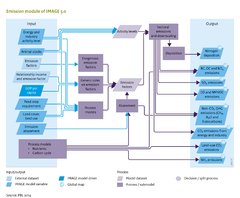
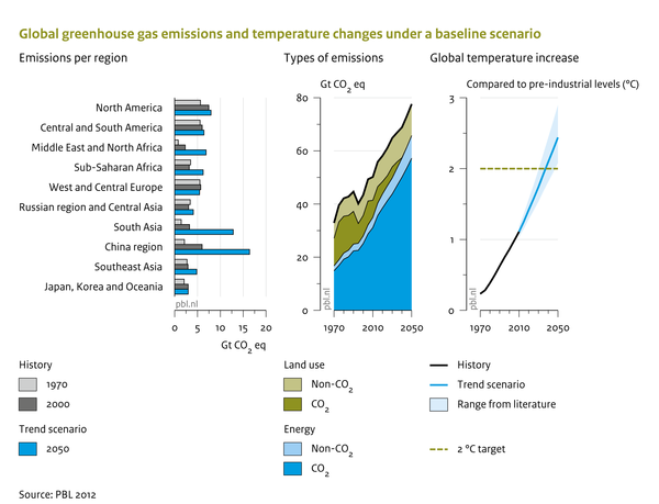
In a baseline scenario, most greenhouse gas ({{abbrTemplate|GHG}}) emissions tend to increase, driven by an increase in underlying activity levels (This is shown in the figure below for a baseline scenario for the [[Roads from Rio+20 (2012) project|Rio+20]] study ([[PBL, 2012]]). Without climate policy, all non-CO<sub>2</sub> {{abbrTemplate|GHG}}s emissions are expected to increase towards the end of the century ([[Lucas et al., 2007]], Harmsen et al., 2019a, [[Harmsen et al., 2019c|2019c]]). For air pollutants, the pattern also depends strongly on the assumptions on air pollution control. In most baseline scenarios, air pollutant emissions tend to decrease, or at least stabilise, in the coming decades as a result of more stringent environmental standards in high and middle income countries. | In a baseline scenario, most greenhouse gas ({{abbrTemplate|GHG}}) emissions tend to increase, driven by an increase in underlying activity levels (This is shown in the figure below for a baseline scenario for the [[Roads from Rio+20 (2012) project|Rio+20]] study ([[PBL, 2012]]). Without climate policy, all non-CO<sub>2</sub> {{abbrTemplate|GHG}}s emissions are expected to increase towards the end of the century ([[Lucas et al., 2007]], Harmsen et al., [[Harmsen et al. 2019a|2019a]], [[Harmsen et al., 2019c|2019c]]). For air pollutants, the pattern also depends strongly on the assumptions on air pollution control. In most baseline scenarios, air pollutant emissions tend to decrease, or at least stabilise, in the coming decades as a result of more stringent environmental standards in high and middle income countries. | ||
{{DisplayPolicyInterventionFigureTemplate|{{#titleparts: {{PAGENAME}}|1}}|Baseline figure}} | {{DisplayPolicyInterventionFigureTemplate|{{#titleparts: {{PAGENAME}}|1}}|Baseline figure}} | ||
==Policy interventions== | ==Policy interventions== | ||
A large variety of mitigation options exist or could be developed to abate emissions from each of the main non-CO<sub>2</sub> GHG emission sources. Lucas et al. (2007), followed by Harmsen et al. (2019c) described the development and application of a set of long-term non-CO2 marginal abatement cost ({{abbrTemplate|MAC}}) curves of all major non-CO<sub>2</sub> GHG sources. These curves represent the mitigation potentials and costs of region- and source-specific mitigation measures and are used in the climate policy module FAIR. The MAC curves have been developed using existing short-term MAC datasets as well as recent literature on emission source-specific mitigation measures. The MAC curves include estimates of future technology development and removal of implementation barriers to capture long-term dynamics. | |||
When applying the new MAC curves to create a 2.6 W/m2 scenario (i.e. likely limiting global warming to 2oC in 2100), the total non-CO2 mitigation was projected to be 10.9 Mt CO2equivalents in 2050 (i.e. 58% reduction compared to baseline emissions) and 15.6 Mt CO2equivalents in 2100 (i.e. a 71% reduction). | |||
The maximum reduction potential (MRP) of all non-CO2 greenhouse gas measures is estimated at 71% in the year 2100. The maximum reduction potential is the highest for F-gases(hydrofluorocarbons (HFCs), perfluorocarbons (PFCs), sulphur hexafluoride (SF<sub>6</sub>), followed by methane (CH<sub>4</sub>) (68%) and nitrous oxide (N<sub>2</sub>O)(62%). CH<sub>4</sub>) emission reductions from (fossil) energy and waste sources are moderately difficult to realize (with reduction potentials between +/- 50% and 80% in 2100). This more the case for emissions from agricultural sources (with reduction potentials between +/- 50% an 70% at very high implementation costs: 3000 – 4000 $/tonne of Carbon). | |||
Maximizing non-CO<sub>2</sub> mitigation is generally a cost-effective strategy in reaching long-term climate targets, but costs vary considerably by source. The curves have been used in the IMAGE IAM framework to derive attractive mitigation strategies. The cost-effectiveness of non-CO2 mitigation varies strongly by emission source. This is shown in Figure 8.2 (lower panel) by plotting the cost of mitigation on the x-axis and the amount of mitigation on the y-axis. As a result, more costly measures are depicted more to the right while sources with a larger absolute reduction potential are depicted more to the top. Mitigation costs for most non-CO2 sources are lower than are lower than those of CO2 mitigation, on average. Note, however, that the mitigation potential of non-CO2 measures is limited and that further mitigation would be far more costly and/or likely not possible. The figure shows that mitigation of HFCs and CH4 from fossil fuel sources can be considered very attractive, due to a large, but relatively low-cost reduction potential. Conversely, reduction of CH4 from wastewater is projected to be relatively costly, due to large infrastructure investments. Here, public health considerations pose a much larger investment incentive than climate. | |||
Policy scenarios present several ways to influence emission of air pollutants ([[Braspenning Radu et al., 2016]]): | Policy scenarios present several ways to influence emission of air pollutants ([[Braspenning Radu et al., 2016]]): | ||
Revision as of 12:57, 5 March 2019
Parts of Emissions/Policy issues
| Component is implemented in: |
Components:and
|
| Projects/Applications |
| Models/Databases |
| Key publications |
| References |
Baseline developments
In a baseline scenario, most greenhouse gas (GHG) emissions tend to increase, driven by an increase in underlying activity levels (This is shown in the figure below for a baseline scenario for the Rio+20 study (PBL, 2012). Without climate policy, all non-CO2 GHGs emissions are expected to increase towards the end of the century (Lucas et al., 2007, Harmsen et al., 2019a, 2019c). For air pollutants, the pattern also depends strongly on the assumptions on air pollution control. In most baseline scenarios, air pollutant emissions tend to decrease, or at least stabilise, in the coming decades as a result of more stringent environmental standards in high and middle income countries.
Policy interventions
A large variety of mitigation options exist or could be developed to abate emissions from each of the main non-CO2 GHG emission sources. Lucas et al. (2007), followed by Harmsen et al. (2019c) described the development and application of a set of long-term non-CO2 marginal abatement cost (MAC) curves of all major non-CO2 GHG sources. These curves represent the mitigation potentials and costs of region- and source-specific mitigation measures and are used in the climate policy module FAIR. The MAC curves have been developed using existing short-term MAC datasets as well as recent literature on emission source-specific mitigation measures. The MAC curves include estimates of future technology development and removal of implementation barriers to capture long-term dynamics.
When applying the new MAC curves to create a 2.6 W/m2 scenario (i.e. likely limiting global warming to 2oC in 2100), the total non-CO2 mitigation was projected to be 10.9 Mt CO2equivalents in 2050 (i.e. 58% reduction compared to baseline emissions) and 15.6 Mt CO2equivalents in 2100 (i.e. a 71% reduction). The maximum reduction potential (MRP) of all non-CO2 greenhouse gas measures is estimated at 71% in the year 2100. The maximum reduction potential is the highest for F-gases(hydrofluorocarbons (HFCs), perfluorocarbons (PFCs), sulphur hexafluoride (SF6), followed by methane (CH4) (68%) and nitrous oxide (N2O)(62%). CH4) emission reductions from (fossil) energy and waste sources are moderately difficult to realize (with reduction potentials between +/- 50% and 80% in 2100). This more the case for emissions from agricultural sources (with reduction potentials between +/- 50% an 70% at very high implementation costs: 3000 – 4000 $/tonne of Carbon).
Maximizing non-CO2 mitigation is generally a cost-effective strategy in reaching long-term climate targets, but costs vary considerably by source. The curves have been used in the IMAGE IAM framework to derive attractive mitigation strategies. The cost-effectiveness of non-CO2 mitigation varies strongly by emission source. This is shown in Figure 8.2 (lower panel) by plotting the cost of mitigation on the x-axis and the amount of mitigation on the y-axis. As a result, more costly measures are depicted more to the right while sources with a larger absolute reduction potential are depicted more to the top. Mitigation costs for most non-CO2 sources are lower than are lower than those of CO2 mitigation, on average. Note, however, that the mitigation potential of non-CO2 measures is limited and that further mitigation would be far more costly and/or likely not possible. The figure shows that mitigation of HFCs and CH4 from fossil fuel sources can be considered very attractive, due to a large, but relatively low-cost reduction potential. Conversely, reduction of CH4 from wastewater is projected to be relatively costly, due to large infrastructure investments. Here, public health considerations pose a much larger investment incentive than climate.
Policy scenarios present several ways to influence emission of air pollutants (Braspenning Radu et al., 2016):
- Introduction of climate policy, which leads to systemic changes in the energy system (less combustion) and thus, indirectly to reduced emissions of air pollutants (Van Vuuren et al., 2006).
- Policy interventions can be mimicked by introducing an alternative formulation of emission factors to the standard formulations (EKC, CLE). For instance, emission factors can be used to deliberately include maximum feasible reduction measures.
- Policies may influence emission levels for several sources, for instance, by reducing consumption of meat products. By improving the efficiency of fertiliser use, emissions of N2O, NO and NH3 can be decreased (Van Vuuren et al., 2011b). By increasing the amount of feed crops in the cattle rations, CH4 emissions can be reduced. Production of crop types has a significant influence on emission levels of N2O, NOx and NH3 from spreading manure and fertilisers.
- Assumptions related to soil and nutrient management. The major factors are fertiliser type and mode of manure and fertiliser application. Some fertilisers cause higher emissions of N2O and NH3 than others. Incorporating manure into soil lowers emissions compared to broadcasting.
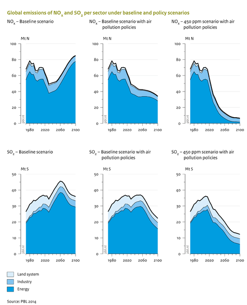
The impacts of more ambitious control policies (CLE versus EKC) on SO2 and NOx, emissions, and the influence of climate policy are presented in the figure below. Where climate policy is particularly effective in reducing SO2 emissions, air pollution control policies are effective in reducing NOx emissions.
See also the Policy interventions Table below.
Effects of policy interventions on this component
| Policy intervention | Description | Effect |
|---|---|---|
| Apply emission and energy intensity standards | Apply emission intensity standards for e.g. cars (gCO2/km), power plants (gCO2/kWh) or appliances (kWh/hour). | |
| Capacity targets | It is possible to prescribe the shares of renewables, CCS technology, nuclear power and other forms of generation capacity. This measure influences the amount of capacity installed of the technology chosen. | |
| Carbon tax | A tax on carbon leads to higher prices for carbon intensive fuels (such as fossil fuels), making low-carbon alternatives more attractive. | |
| Change market shares of fuel types | Exogenously set the market shares of certain fuel types. This can be done for specific analyses or scenarios to explore the broader implications of increasing the use of, for instance, biofuels, electricity or hydrogen and reflects the impact of fuel targets. (Reference:: Van Ruijven et al., 2007) | |
| Change the use of electricity and hydrogen | It is possible to promote the use of electricity and hydrogen at the end-use level. | |
| Excluding certain technologies | Certain energy technology options can be excluded in the model for environmental, societal, and/or security reasons. (Reference:: Kruyt et al., 2009) | |
| Implementation of biofuel targets | Policies to enhance the use of biofuels, especially in the transport sector. In the Agricultural economy component only 'first generation' crops are taken into account. The policy is implemented as a budget-neutral policy from government perspective, e.g. a subsidy is implemented to achieve a certain share of biofuels in fuel production and an end-user tax is applied to counterfinance the implemented subsidy. (Reference:: Banse et al., 2008) | |
| Implementation of sustainability criteria in bio-energy production | Sustainability criteria that could become binding for dedicated bio-energy production, such as the restrictive use of water-scarce or degraded areas. | |
| Improving energy efficiency | Exogenously set improvement in efficiency. Such improvements can be introduced for the submodels that focus on particular technologies, for example, in transport, heavy industry and households submodels. | |
| REDD policies | The objective of REDD policies it to reduce land-use related emissions by protecting existing forests in the world; The implementation of REDD includes also costs of policies. (Reference:: Overmars et al., 2012) | Less emissions due to deforestation and land-use change. |