Drivers/Model drivers

Projects/Applications

IPCC SRES (2000) project Millennium Ecosystem Assessment - MA (2005) project OECD Environmental Outlook to 2050 (2012) project Shared Socioeconomic Pathways - SSP (2014) project

Models/Databases

ENV-Growth model MAGNET model

Relevant overviews

Framework overview Policy interventions and components overview Variable overview

Key publications

IPCC, 2000 MA, 2005 OECD, 2012

References

Alexandratos and Bruinsma, 2012 Bouwman et al., 2005 Bouwman et al., 2013b Bruinsma, 2003 FAO, 2013a Klein Goldewijk et al., 2010 Mulders et al., 2006 Rogner, 1997 Rohwer et al., 2007

Flowchart Drivers. Model drives are inferred from scenario storylines taking into account external data sources, such as time series, cross-sector data, and literature sources.

Model drivers

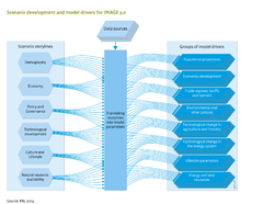
Direct model drivers are inferred from the scenario drivers and used in setting the parameter values in IMAGE 3.0. The start values are estimated from the literature and data, and future changes in values are inferred from the narratives and scenario drivers. The resulting parameter values are used as input for different parts of IMAGE 3.0. A list of most important model drivers, their source and their use in Framework overviewis given in the table of drivers below.

Example of a model driver: technological change in agriculture

The management factor (MF) describes the actual yield per crop group and per socio-economic region as a proportion of the maximum potential yield. This maximum potential yield is estimated taking into account inhomogeneous soil and climate data across grid cells. The MF for the period up to 2005 is estimated as part of the IMAGE calibration procedure, using FAO statistics on actual crop yields and crop areas (FAO, 2013a). The start year for the MF is subsequently taken as point of departure for future projections.

Guidance for future development of yield changes is provided by expert projection such as the assumptions in FAO projections up to 2030 and 2050 (Bruinsma, 2003; Alexandratos and Bruinsma, 2012).The FAO trends are used as exogenous technical development in the MAGNET model, and subsequently adjusted to reflect the relative shortage of suitable land, as part of the model calculation (Component Agricultural economy). The combinations of production volumes and land areas from MAGNET are adopted as future MF projections into the future in IMAGE.

Future technological change is dependent on the storyline and needs to be consistent with other scenario drivers. For instance, strong economic growth is typically facilitated by rapid technology development and deployment, rising wages and a labour shift from primary production (agriculture) to secondary (industry) and tertiary (services) sectors. These developments foster more advanced management and technology in agriculture. In order to reflect different trends in exogenous yield increase, FAO trends are combined with projections of economic growth to develop scenario-specific trends of yield changes in multiple—baseline studies, like for the SSPs. Because the MF is such a decisive factor in future net agricultural land area, careful consideration of uncertainties is warranted.

|Table=

Table of drivers

Driver	Description	Source	Use
Population projections
Population	Number of people per region.	UN future: exogenous input	Energy supply and demand Agricultural economy Climate policy Energy demand
Population - grid	Number of people per gridcell (using downscaling).	UN own downscaling	Land-use allocation Nutrients Human development Flood risks
Urban population fraction	Urban/rural split of population.	UN future: exogenous input	Human development
Economic development
Capital supply	Capital available to replace depreciated stock and expand the stock to support economic growth.	GTAP database	Agricultural economy
GDP per capita	Gross Domestic Product per capita, measured as the market value of all goods and services produced in a region in a year, and is used in the IMAGE framework as a generic indicator of economic activity.	World Bank database future: exogenous input	Energy supply and demand Agricultural economy Climate policy Emissions Energy demand Human development
GDP per capita - grid	Scaled down GDP per capita from country to grid level, based on population density.	Own downscaling	Ecosystem services Nutrients Flood risks
GINI coefficient	Measure of income disparity in a population. If all have the same income, GINI equals 1. The lower the GINI, the wider the gap between the lowest and highest income groups.	World Bank database future: scenario assumptions	Human development
Labour supply	Effective supply of labour input to support economic activities, taking into account the participation rate of age cohorts.	Demographics: population by age cohort times participation rate, corrected for skill level	Agricultural economy
Private consumption	Private consumption reflects expenditure on private household consumption. It is used in IMAGE as a driver of energy.	The World Bank future: exogenous input	Energy supply and demand Energy demand
Sector value added	Value Added for economic sectors: Industry (IVA), Services (SVA) and Agriculture (AVA). These variables are used in IMAGE to indicate economic activity.	Various sources	Energy supply and demand Energy demand
Timber demand	Demand for roundwood and pulpwood per region.	FAO future: exogenous input or own calculation	Forest management
Trade regimes, tariffs and barriers
Trade policy	Assumed changes in market and non-market instruments that influence trade flows, subject to WTO rules and country and region regulation.	Own assumptions	Agricultural economy
Trade restriction	Trade tariffs and barriers limiting trade in energy carriers (in energy submodel).	Own assumptions	Energy supply
Environmental and other policies
Adaptation level	Level of adaptation to climate change , defined as the share of climate change damage avoided by adaptation. This level is be calculated by the model to minimise adaptation costs and residual damage, or set by the user.	own assumpions, optimisation	Climate policy
Air pollution policy	Air pollution policies set to reach emission reduction targets, represented in the model in the form of energy carrier and sector specific emission factors.	EDGAR database future based on own assumptions	Energy conversion
Biofuel policy	Policies to foster the use of biofuels in transport, such as financial incentives and biofuel mandates and obligations.	Literature and own assumptions	Agricultural economy
Climate target	Climate target, defined in terms of concentration levels, radiative forcing, temperature targets, or cumulative emissions.	Own assumptions	Climate policy
Domestic climate policy	Planned and/or implemented national climate and energy policies, such as taxes, feed-in tariffs, renewable targets, efficiency standards, that affect projected emission reduction.	Own assumptions	Climate policy
Energy policy	Policy to achieve energy system objectives, such as energy security and energy access.	Own assumptions	Energy conversion
Equity principles	General concepts of distributive justice or fairness used in effort sharing approaches. Three key equity principles are: Responsibility (historical contribution to warming); capability (ability to pay for mitigation); and equality (equal emissions allowances per capita).	Expert judgement	Climate policy
Protected area - grid	Map of protected nature areas, limiting use of this area.	WDPA database own assumptions, derived from polygon maps	Land-use allocation Land cover and land use Terrestrial biodiversity Ecosystem services
Taxes and other additional costs	Taxes on energy use, and other additional costs	IEA future: scenario assumptions	Energy demand
Technological change in the energy system
Energy efficiency technology	Model assumptions determining future development of energy efficiency.	Own assumptions	Energy demand
Energy intensity parameters	Set of parameters determining the energy use per unit of economic activity (in absence of technical energy efficiency improvements).	IEA future: own calculations and scenario assumptions	Energy demand
Learning rate	Determines the rate of technology development in learning equations.	Literature and scenario assumptions	Energy supply
Technology development of energy conversion	Learning curves and exogenous learning that determine technology development.	Scenario assumption based on various sources	Energy supply and demand Energy conversion
Technology development of energy supply	Learning curves and exogenous learning that determine technology development.	Scenario assumptions based on various sources	Energy supply and demand Energy supply
Energy and land resources
Built-up area - grid	Urban built-up area per grid cell, excluded from all biophysical modelling in IMAGE, increasing over time as a function of urban population and a country- and scenario-specific urban density curve.	Klein Goldewijk et al., 2010	Land cover and land use
Energy resources	Volume of energy resource per carrier, region and supply cost class (determines depletion dynamics).	Mulders et al., 2006, Rogner, 1997	Energy supply and demand Energy supply
Technological change in agriculture and forestry
Animal productivity	Effective production of livestock commodities per animal per year.	FAOSTAT database future: scenario assumptions	Livestock systems
Feed conversion	Measure of an animal's efficiency in converting feed mass into the desired output such as meat and milk (for cattle, poultry, pigs, sheep and goats).	FAOSTAT database future: scenario assumptions	Livestock systems
Fertiliser use efficiency	Ratio of fertiliser uptake by a crop to fertiliser applied.	FAOSTAT database future: scenario assumptions Bouwman et al., 2013b	Nutrients
Forest plantation demand	Demand for forest plantation area.	FAOSTAT database future: scenario assumptions	Forest management
Fraction of selective logging	The fraction of forest harvested in a grid, in clear cutting, selective cutting, wood plantations and additional deforestation. Fraction of selective cut determines the fraction of timber harvested by selective cutting of trees in semi-natural and natural forest.	Own estimates, based on FAO	Forest management
Harvest efficiency	Fraction of harvested wood used as product, the remainder being left as residues. Specified per biomass pool and forestry management type.	Various sources	Forest management
Increase in irrigated area - grid	Increase in irrigated area, often based on external projections (e.g., FAO).	FAO, IIASA Own assumptions for spatial allocation	Land-use allocation
Irrigation conveyance efficiency	Ratio of water supplied to the irrigated field to the quantity withdrawn from the water source, determining the quantity of water lost during transport. This parameter is defined at country level.	PIK Rohwer et al., 2007
Irrigation project efficiency	Ratio of quantity of irrigation water required by the crop (based on soil moisture deficits) to the quantity withdrawn from rivers, lakes, reservoirs or other sources. This parameter is given at country level.	PIK Rohwer et al., 2007
Livestock rations	Determines the feed requirements per feed type (food crops; crop residues; grass and fodder; animal products; scavenging), specified per animal type and production system (extensive/intensive/backyard/intermediate/intensive/broiler/laying hens).	Own estimates Bouwman et al., 2005, Lassaletta et al., 2019	Livestock systems Nutrients
Manure spreading fraction	Fraction of manure produced in staples that is spread on agricultural areas.	Own estimates Bouwman et al., 2013b	Nutrients
Production system mix	Livestock production is distributed over two systems for dairy and beef production (intensive: mixed and industrial; extensive: pastoral grazing), and to three systems for pigs (backyard, intermediate, intensive) and poultry (backyard, boilers, laying hens) with specific intensities, rations and feed conversion ratios.	Own estimates Bouwman et al., 2005, Lassaletta et al., 2019	Livestock systems Nutrients
Technological change (crops and livestocks)	Increase in productivity in crop production (yield/ha) and livestock production (carcass weight, offtake rate).	FAO own estimates	Agricultural economy
Lifestyle parameters
Lifestyle parameters	Lifestyle parameters influence the relationship between economic activities and demand for energy.	IEA based on calibration	Energy supply and demand Energy demand
Preferences	Non-price factors determining market shares, such as preferences, environmental policies, infrastructure and strategic considerations, used for model calibration.	Calibration, future: scenario assumptions	Energy demand